Curvature Beziers
Improving on a timeless recipe

The bezier curve is a staple of CAD and computer graphics. Like Bic pens, the design is decades old and they're everywhere. You'll often find them as the default or only choice in various illustration and animation tools.
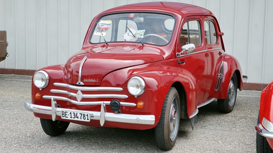
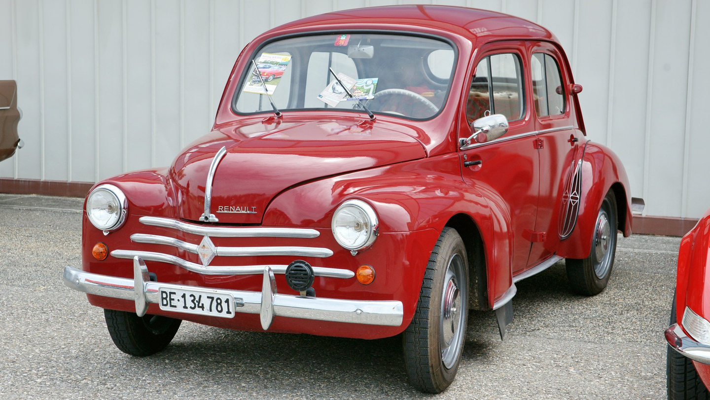
Conceived by Paul de Casteljau in 1959, and refined by Pierre Bézier in the 1960s at Renault, the enduring appeal of the bezier curve lies in its simplicity. While more sophisticated curves have been invented, and new ones continue to be proposed, these are limited to specific domains, like high-precision CAD or road design. In general use, the bezier stubbornly refuses to be dethroned, despite its shortcomings.
Hence bezier curves are a piece of legacy tech we appear to be stuck with. As a software engineer, my question then is: can we make beziers better without invalidating all the tech built on and with them?
The answer is yes.
Lerp-a-derp
Drawing a bezier curve is a surprisingly simple and linear process:
Tip: All the diagrams in this post are fully interactive.
Given a series of control points, we connect them with lines. We then run along those lines simultaneously, to produce new points, which can be connected again. This process is repeated until we are left with a single point, which lies on the curve.
This construction makes beziers far more regular than they might first appear.
The linear interpolations (aka lerps) can be summarized into a single compact formula, e.g. for 4 control points $ \left(A, B, C, D\right) $:
The rule is simple: descending powers of $\left(1 - t\right)$, ascending powers of $t$, with coefficients taken from the n'th row of Pascal's triangle:
For curves in 2D and 3D, the formula is applied to the individual X, Y or Z coordinates.
While beziers can be constructed for any number of control points, the common practice is to only use cubic beziers with 4 control points. This is because the curve is only guaranteed to cross through the first and last control point, which makes higher degree beziers more difficult to shape.
Larger curves are instead constructed by joining together multiple cubic bezier segments, with the tangents lined up to create a segmented curve that appears smooth:
This is the cubic bezier spline, as commonly understood. The precision "pen tool" in most drawing apps then consists of drawing and editing the control points, rather than drawing curves directly.
A Lie Told Everywhere
Pen tools typically have a few different modes for the control points:
Intuitively these represent various degrees of smoothness. Symmetric tangents are offered as the smoothest option, with some qualities of smoothness being lost as you relax the constraints.
In reality this is completely wrong, and this is easy to demonstrate.
Bezier curves can be split exactly, by reading off the new control points from the interpolation diagram:
The left and right segments are 100% identical to the original curve, and always join up perfectly at the seam. Yet the tangents in the middle will be asymmetric except for one split near the middle. This can be confirmed using a curvature comb which represents the (inverse) radius of curvature at every point:
The curvature comb remains continuous, with no jumps.
This means that whether or not adjacent tangents are of equal length, i.e. symmetric, is completely irrelevant. Attempting to draw smooth and intuitive bezier curves this way is a fool's errand.
A simple way to improve this is to treat the tangents as relative rather than absolute. e.g. We can make them proportional to the distance between the start and end of each segment:
This spline is easier to edit, because as you move each curve point around, the adjacent segments naturally flex to get out of the way. There are far fewer cusps created this way. Editing the tangents remains the same.
However if we plot curvature again, we can tell this isn't a great solution:
Scaling tangents proportionally doesn't guarantee that curvature is preserved, nor does curvature remain continuous from one segment to the next.
This also shows that offering users a curvature comb visualization as a "helpful tool" is really quite mean: adjusting the curvature on one end will also affect the other side, requiring repeated adjustments back and forth until it's close enough.
Handle Carefully
A much more effective strategy is to work with curvature directly.
While this is a difficult problem in general, it turns out there are some surprising relationships here, which we can observe directly:
Consider the curvature at the start of segment $A-B-C-D$. This is affected only by the positions of $A$, $B$ and $C$. Point $D$ can be moved freely if it's detached from $C$.
Furthermore, because the tangent $A-B$ is horizontal, only the vertical position of $C$ matters. This is a result of the underlying linear interpolations, which end up cancelling out a lot of terms in the formulas.
The curvature at $A$ is therefor only affected by the length of $A-B$, and the perpendicular distance from $C$ to $A-B$. The same applies to $D$ on the other side with $C-D$ and $B$.
This isn't very useful by itself though. When we move a curve point ($A$ or $D$), typically the adjacent control point ($B$ or $C$) is moved as well to preserve the tangent. And when we turn a symmetric or asymmetric tangent, the adjacent tangent in the next segment is turned by the same angle, altering the curvature on that side.
Still, this shows that preserving curvature is not by itself a crazy idea and can be done simply by scaling the tangents appropriately. The rules would be simple:
When we move a curve point, we have to preserve the start and end curvature in the adjacent segments
When we move a tangent, we have to preserve the curvature on the opposite end of the current segment, as well as on both sides of the adjacent segment
This ought to produce an editing experience where the curve actually respects your intent. Except not quite:
Moving curve points works great, but when turning a tangent, the length of that tangent is itself a poor representation of the user's intent. Small changes can cause huge shifts in curvature, which can cause the curve to jump around and explode unexpectedly as it tries to find a matching solution.
Hence it's better to work with curvature handles instead, where the length corresponds directly to curvature:
Unlike the curvature comb, the length of the handles is the non-inverted radius of curvature, which is the more natural choice.
These handles are very stable and can be converted just-in-time to classic bezier control points, without needing to round-trip back and forth between the two representations. Helpfully, this also avoids numerical drift.
Goldilocks
To actually pull this off, we need to solve for the lengths $l_0$ and $l_1$ of the tangents, given the desired curvatures $k_0$ and $k_1$, the start/end points $A$ and $D$, and the unit-length tangents at the start/end.
Given a curve $\gamma\left(t\right)$, we can express the unit tangent vector $\mathbf{T}\left(t\right)$ as the normalized derivative:
This can be used to find the curvature vector $\mathbf{K}\left(t\right)$ via two vector cross products using the first and second derivative:
The cross products ensure that $\mathbf{K}\left(t\right)$ is perpendicular to $\mathbf{T}\left(t\right)$, i.e. they extract the normal vector component of the middle term. Now we can solve for $\mathbf{K}\left(0\right) = k_0$ and $\mathbf{K}\left(1\right) = k_1$.
After working through the math, we end up with a quadratic system of equations in $l_0$ and $l_1$:
Where:
This captures a few things:
The sign of the curvature $k_i$ defines whether the curve turns clockwise or counterclockwise. When moving curve points around, the curve may be forced to flip, hence the $±$ is necessary, and both signs can change independently.
The coupling between $l_0$ and $l_1$ is influenced only by $b$. If $b = 0$, then the two equations are independent and the problem is trivial to solve. This corresponds to the situation where the two tangents are parallel.
The constant term $c_i$ is influenced only by the perpendicular distance $D - A$ (or $A - D$) to the tangent $\mathbf{T_i}$. This matches the earlier finding that only perpendicular distance affects curvature.
Hence, the problem is reduced to finding the intersection of two double-parabolas, one horizontal and one vertical:
The two sides of each double-parabola represent bending clockwise or counterclockwise. We have to solve 4 times, one for each sign combination $\left(+,+\right)$, $\left(+,-\right)$, $\left(-,+\right)$, $\left(-,-\right)$.
To solve this system, we can rewrite either of the equations to isolate $l_1$ or $l_0$:
Pick one, and square it to plug it into the other original equation as the $l_1^2$ or $l_0^2$ term. This produces a quartic equation in the other variable (resp. $l_0$ or $l_1$), which can be solved directly using the quartic formula.
We can then compute the other $l_i$, either:
Not all solutions of the quartic will be actual solutions to the system however, because of the squaring. So we have to double check that the original equations hold before accepting a solution for $\left(l_0, l_1\right)$.
We also want to reject solutions where $l_0 < 0$ or $l_1 < 0$, because these represent situations where the tangents have been flipped by 180º.
In most cases, there will only be one valid solution, and this works pretty well:
For corner-type points, one or both $k_i$'s are infinite. This is straightforward to solve as the matching $l_i$ is zero and the other can be computed directly.
Grouper and Snapper
Unfortunately if there are multiple solutions, these each represent a different curve:
Having the curve jump around as you edit it would be a very bad editing experience, but there is no obvious way to pick the right one.
One strategy would be to remember the previous $l_0$ and $l_1$ as you edit, and pick the solution that is closest to the previous curve. However this would introduce path-dependence into editing, where the order and direction that you moved points around in affects which curve you end up with. For a drawing tool, this is quite frustrating and undesirable.
Different solutions to the equation can also appear and vanish suddenly, so this wouldn't eliminate popping either, merely reduce it.
Ideally the resulting curvatures should always change smoothly themselves. This can be accomplished by designing an appropriate weighting heuristic for the solutions, and calculating their weighted average.
1) The forbidden regions:
When a solution approaches either $l_0 < 0$ or $l_1 < 0$, it's about to vanish, so its weight should go to zero there.
2) When two opposite-bending parabolas are about to become tangent, two solutions will move towards each other, before both vanishing at the same time:
These solutions are unstable and should be avoided. To detect this, I calculate the gradient vector of each equation.
The angle between them can be found via their dot product, after dividing by their respective lengths:
A value close to $-1$ means two opposite-bending parabolas, while a value close to $1$ means two aligned parabolas. The latter is not as bad, as this implies many almost-equivalent solutions.
3) When the radius of curvature is very big compared to the bezier itself, one of the possible solutions is for the curve to cross through itself, forming a loop. This should be discouraged:
We can divide by the length of $|\mathbf{l}|$ i.e. $\sqrt{l_0^2 + l_1^2}$, preferring solutions that have shorter tangents.
Putting it all together, the weighting heuristic I chose is:
By applying $\arccos \left(-\cos \theta\right)$, we remap the dot-product range $(-1..1)$ to $(0..π)$ which effectively neutralizes the unstable solutions
Large $|\mathbf{l}|$'s represent undesirable solutions, so should be strongly penalized and only chosen if they are the only option
When the entire heuristic approaches $0$, the influence should vanish smoothly, hence the overall squaring
Using this as the weight, the resulting bezier curves always change smoothly, even when the start and end are moved around and through each other.
But when multiple solutions are averaged together, the resulting $(l_0, l_1)$ is not necessarily a solution to the original system. This means the resulting curvatures are not always exact, even when there is an exact solution nearby.
To mitigate this, we can add an additional resampling step, where we re-weigh the solutions according to the inverse distance^4 to the weighted average:
This causes the solution to snap smoothly to exact solutions when available.
Migratory Curves
What's especially nice about this approach is that it can largely be slotted into existing systems with little modification required.
The UI of adjusting and editing bezier handles can be kept, including the notion of the 4 point types. Just the meaning of the lengths of the tangents changes. Converting an asymmetric point to a symmetric point will actually equalize the curvature of the left and right side, which is what the user actually wants.
The internal representation can mostly remain the same type, i.e. a series of points, just those points represent curvature tangents, not bezier tangents. Though it's better to explicitly store the unit length tangents and curvatures directly, which is more numerically stable. For the demos here I made pairwise conversion functions between curvature handles ↔︎ points/tangents/curvatures ↔︎ bezier handles.
Splitting a curvature bezier is a lot simpler than splitting a classic bezier, because the start and end handles don't change at all, and the newly created handles are symmetric:
There is one remaining flaw though. When splitting a curve with an S-bend, the splits near the bend are not exact:
The heuristic picks the wrong curve on one or both sides. This can be fixed by remembering the specific orientation of the curvature, and only flipping the curvature sign when necessary. Though this does introduce some minimal path-dependence into editing.
So really you would need to expose this in the UI as an extra orientation toggle for ambiguous control points. It would also mean that the internal representation has to be in tangent + signed curvature form to be fully stable, not just curvature handles.
Near the S-bend, the radius of curvature—and thus the handle size—effectively becomes infinite, because $|k|$ becomes $0$. The bezier control points lie on a straight line, as perpendicular distance to the tangent is zero.
So even when handled exactly, this can still create impractically large curvature handles. Perhaps what's needed is a 5th "Inflection" point type, for points with exactly zero $|k|$, though such points tend to be very unstable, and sometimes no solution exists:
To migrate a classic bezier to a curvature bezier, you can measure the unit tangents and curvature at the start and end. In the vast majority of cases this will result in the exact same curve. If it doesn't, then you must split the original bezier to avoid the ambiguity.
For complex operations on bezier curves, e.g. boolean union or intersection, these still have to be done in bezier form. This implies some amount of round-tripping between the two representations, which would introduce numerical drift. However, only the newly created points need to be converted back, because the curvature and tangents elsewhere remain the same.
* * *
This post started from the observation that "symmetric" bezier tangents aren't actually symmetric as you'd expect. Hopefully you found the resulting exploration enlightening.
The practice of showing curvature combs to diagnose problems with splines is really backwards. If we can show a curvature comb, we can also compute an appropriate spline to match the desired curvature.
So beziers as they commonly exist are quite inadequate. We can retrofit a better system to edit them without breaking the expectations of a smooth editing experience, or introducing a new class of curves that behaves very differently.
The code for the diagrams and implementation can be found on GitLab.