It's been over two months since the last installment in this series. Oops. Unfortunately, while trying to get to the next stage of this project, I ran into some walls. My main problem is that I'm not just creating worlds, but also learning to work with the Ogre engine and modern graphics hardware in particular.

This presents some interesting challenges: between my own code and the pixels on the screen, there are no less than three levels of indirection. First, there's Ogre, a complex piece of C++ code that provides me with high-level graphics tools (i.e. objects in space). Ogre talks to OpenGL, which abstracts away low-level graphics operations (i.e. commands necessary to draw a single frame). The OpenGL calls are handed off to the graphics driver, which translates them into operations on the actual hardware (processing vertices and pixels in GPU memory). Given this long dependency chain, it's no surprise that when something goes wrong, it can be hard to pinpoint exactly where the problem lies. In my case, an oversight and misunderstanding of an Ogre feature lead to several days of wasted time and a lot of frustration that made me put aside the project for a while.

With that said, back to the planets...

Normal mapping

Last time, I ended with a bumpy surface, carved by applying brushes to the surface. The geometry was there, but the surface was still just solid white. To make it more visually interesting, I'm going to apply light shading.

The most basic information you need for shading a surface is the surface normal. This is the vector that points straight away from the surface at a particular point. For flat surfaces, the normal is the same everywhere. For curved surfaces, the normal varies continuously across the surface. Typical materials reflect the most light when the surface normal points straight at the light source. By comparing the surface normal with the direction of incoming light (using the vector dot product), you can get a good measure of how bright the surface should be under illumination:

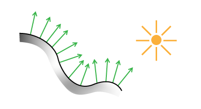Lighting a surface using its normals.

To use normals for lighting, I have two options. The first is to do this on a geometry basis, assigning a normal to every triangle in the planet mesh. This is straightforward, but ties the quality of the shading to the level of detail in the geometry. A second, better way is to use a normal map. You stretch an image over the surface, as you would for applying textures, but instead of color, each pixel in the image represents a normal vector in 3D. Each pixel's channels (red, green, blue) are used to describe the vector's X, Y and Z values. When lighting the surface, the normal for a particular point is found by looking it up in the normal map.

The benefit of this approach is that you can stretch a high resolution normal map over low resolution geometry, often with almost no visual difference.

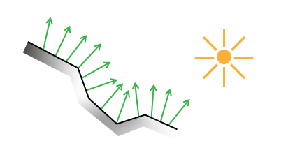Lighting a low-resolution surface using high-resolution normals.

Here's the technique applied to a real model:

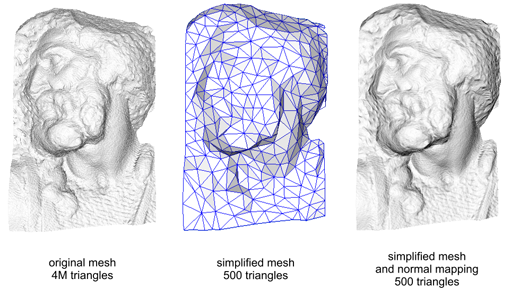(Source - Creative Commons Share-alike Attribution)

Normal mapping helps keep performance up and memory usage down.

Finding Normals

So how do you generate such a normal map, or even a single normal at a single point? There are many ways, but the basic principle is usually the same. First you calculate two different vectors which are tangent to the surface at the point in question. Then you use the cross product to find a vector perpendicular to the two. This third vector is unique and will be the surface normal.

For triangles, you can pick any two triangle edges as vectors. In my case, the surface is described by a heightmap on a sphere, which makes things a bit trickier and requires some math.

I asked my friend Djun Kim, Ph.D. and teacher of mathematics at UBC for help and he recommended Calculus on Manifolds by Michael Spivak. This deceptively small and thin book covers all the basics of calculus in a dense and compact way, and quickly became my new favorite reading material.

Differential Geometry

In this section, I'll describe the formulas needed to calculate the normals of a spherical heightmap. Unlike what I've written before, this will dive shamelessly into specifics and not eschew math. The reason I'm writing it down is because I couldn't find a complete reference online. If math scares you, this section might not be for you. Scroll down until you reach the crater, or take a detour by reading A Mathematician's Lament by Paul Lockhart, which will enlighten you.

First, we're going to derive normals for a regular flat terrain heightmap. To start, we need to define the terrain surface. Starting with a 2D heightmap, i.e. a function f(u,v) of two coordinates that returns a height value, we can create a 3 dimensional surface g:

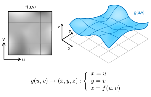
We can use this formal description to find tangent and normal vectors. A vector is tangent when its direction matches the slope of the surface in a particular direction. Differential math tells us that slope is found by taking the derivative. For our function of 2 variables, that means we can find tangent vectors along curves of constant v or constant u. These curves are the thin grid lines in the diagram. Actually, we can find tangents along any line, in any direction. But along u and v lines, the other variable acts like a constant, which simplifies things.

To do this, we take partial derivatives with respect to u (with v constant) and with respect to v (with u constant). The set of all partial derivatives is called the Jacobian matrix J, whose rows form the tangent vectors t_u and t_v, indicated in red and purple:

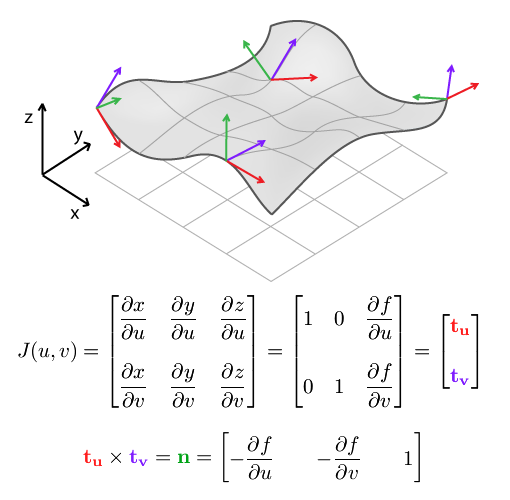
The cross product of t_u and t_v gives us n, the surface normal.

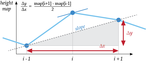
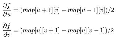
When applied to a discrete heightmap, the function f(u,v) is a 2D array map[u][v], and the partial derivatives at the end have to be replaced with something else. We can use finite differences to approximate the slope of the surface by differencing neighbouring samples:

This result and the formula for n are usually provided as-is in terrain mapping guides, without going through the full process of finding tangents first. However, it's important to use the Jacobian matrix formulation once you switch to spherical terrain.

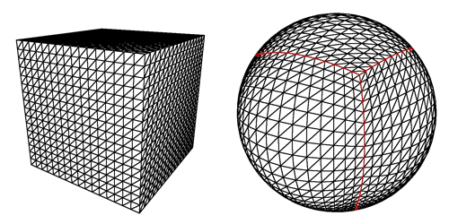
To make a sphere, we add an additional function k which warps the flat terrain into a spherical shell. Each shell is the result of warping a single face of the cubemap and covers exactly 1/6th of the sphere. In what follows, We'll only consider a single face and its shell.

We designate the intermediate pre-warp coordinates (s,t,h), and the final post-warp coordinates as (x,y,z):

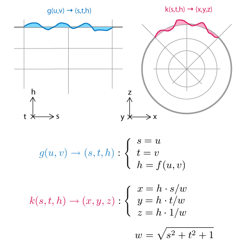
The principle behind the spherical mapping is this: first we take the vector (s, t, 1), which lies in the base plane of the flat terrain. We normalize this vector by dividing it by its length w, which has the effect of projecting it onto the sphere: (s/w, t/w, 1/w) will be at unit distance from (0, 0, 0). Then we multiply the resulting vector by the terrain height h to create the terrain on the sphere's surface, relative to its center: (h·s/w, h·t/w, h/w)

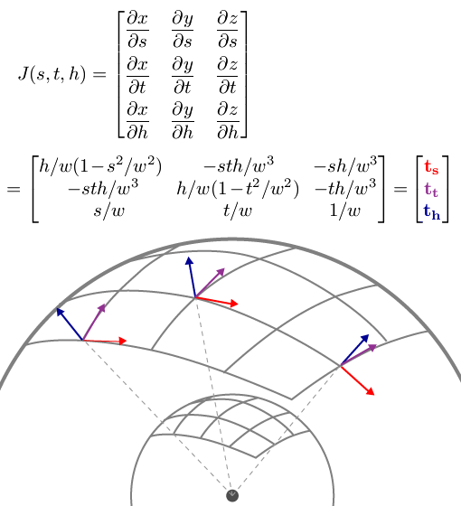
Just like with the function g(u,v) and J(u,v), we can find the Jacobian matrix J(s,t,h) of k(s,t,h). Because there are 3 input values for the function k, there are 3 tangents, along curves of varying s (with constant t and h), varying t (constant s and h) and varying h (constant s and t). The three tangents are named t_s, t_t, t_h.

PS: If your skills at derivation are a bit rusty, remember that Wolfram Alpha can do it for you.

How does this help? The three vectors describe a local frame of reference at each point in space. Near the edges of the grid, they get more skewed and angular. We use these vectors to transform the flat frame of reference into the right shape, so we can construct a new 90 degree angle here.

In mathematical terms, we multiply the 'flat' partial derivatives by the Jacobian matrix. This is similar to the chain rule for regular derivatives, only for multiple variables.

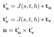
That is, to find the partial derivatives (i.e. tangent vectors) of the final spherical terrain with respect to the original terrain coordinates u and v, we can take the flat terrain's tangents t_u and t_v and multiply them by J(s,t,h). Once we have the two post-warp tangents, we take their cross product, and find the normal of the spherical terrain:

It's imporant to note that this is not the same as simply multiplying the flat terrain normal with J(s,t,h). J(s,t,h)'s rows do not form a set of perpendicular vectors (it is not an orthogonal matrix), which means it does not preserve angles between vectors when you multiply by it. In other words, J(s,t,h) * n, with n the flat terrain normal, would not be perpendicular to the spherical terrain. This is why it's important to return to the basic calculus underneath, so we can get the correct, complete formula.

Thus ends the magical math adventure. If you read it all the way through, cheers!

No Wait, It is a Moon.

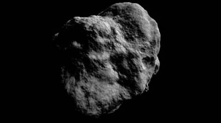
With the normal map in place, I can now render the planet's surface and get a realistic idea of what it looks like. To show this off, I tweaked the brush system a bit: instead of using the literal brush image (e.g. a smooth, round crater), the brush is distorted with fractal noise. It makes every application of the brush subtly different from the next, and saves me from manually drawing e.g. a hundred different craters.

Here's a side by side comparison of the original brush and a distorted version.

Currently I've only implemented one type of distortion, which lends a rocky appearance to the surface. With that in place, my engine can now generate somewhat realistic looking moon surfaces. Here's the demo:

References

The techniques I used were pioneered by people smarter and older than me, I'm just building my own little digital machine with them.

• Creating Spherical Worlds, Maxis/Electronic Arts. (source).
• Calculus on Manifolds, Michael Spivak.