August 06, 2010

My JS1K Demo - The Making Of

Now, whenever size is an issue, the best way to make a small program is to generate all data on the fly, i.e. procedurally. This saves valuable storage space. While this might seem like a black art, often it just comes down to clever use of (high school) math. And as is often the case, the best tricks are also the simplest, as they use the least amount of code.

To illustrate this, I'm going to break down my demo and show you all the major pieces and shortcuts used. Unlike the actual 1K demo, the code snippets here will feature legible spacing and descriptive variable names.

Initialization

JS1K's rules give you a Canvas tag to work with, so the first piece of code initializes it and makes it fill the window.

From then on, it just renders frames of the demo. There are four major parts to this:

• Animating the wires
• Rotating and projecting the wires into the camera view
• Coloring the wires
• Animating the camera

All of this is done 30 times per second, using a normal setInterval timer:

setInterval(function () { ... }, 33);

Drawing Wires

The most obvious trick is that everything in the demo is drawn using only a single primitive: a line segment of varying color and stroke width. This allows the whole drawing process to be streamlined into two tight, nested loops. Each inner iteration draws a new line segment from where the previous one ended, while the outer iteration loops over the different wires.

The lines are blended additively, using the built-in 'lighten' mode, which means they can be drawn in any order. This avoids having to manually sort them back-to-front.

To simplify the perspective transformations, I use a coordinate system that places the point (0, 0) in the center of the canvas and ranges from -1 to 1 in both coordinates. This is a compact and convenient way of dealing with varying window sizes, without using up a lot of code:

with (graphics) {
  ratio = width / height;
  globalCompositeOperation = 'lighter';
  scale(width / 2 / ratio, height / 2);
  translate(ratio, 1);
  lineWidthFactor = 45 / height;
  ...

I add a correction ratio for non-square windows and calculate a reference line width lineWidthFactor for later. Here, I'm using the with construct to save valuable code space, though its use is generally discouraged.

Then there's the two nested for loops: one iterating over the wires, and one iterating over the individual points along each wire. In pseudo-code they look like:

For (12 wires => wireIndex) {
  Begin new wire
  For (45 points along each wire => pointIndex) {
    Calculate path of point on a sphere: (x,y,z)
    Extrude outwards in swooshes: (x,y,z)
    Translate and Rotate into camera view: (x,y,z)
    Project to 2D: (x,y)
    Calculate color, width and luminance of this line: (r,g,b) (w,l)
    If (this point is in front of the camera) {
      If (the last point was visible) {
        Draw line segment from last point to (x,y)
      }
    }
    else {
      Mark this point as invisible
    }
    Mark beginning of new line segment at (x,y)
  }
}

Mathbending

To generate the wires, I start with a formula which generates a sinuous path on a sphere, using latitude/longitude. This controls the tip of each wire and looks like:

offset = time - pointIndex * 0.03 - wireIndex * 3;
longitude = cos(offset + sin(offset * 0.31)) * 2
          + sin(offset * 0.83) * 3 + offset * 0.02;
latitude = sin(offset * 0.7) - cos(3 + offset * 0.23) * 3;

This is classic procedural coding at its best: take a time-based offset and plug it into a random mish-mash of easily available functions like cosine and sine. Tweak it until it 'does the right thing'. It's a very cheap way of creating interesting, organic looking patterns.

This is more art than science, and mostly just takes practice. Any time spent with a graphical calculator will definitely pay off, as you will know better which mathematical ingredients result in which shapes or patterns. Also, there are a couple of things you can do to maximize the appeal of these formulas.

First, always include some non-linear combinations of operators, e.g. nesting the sin() inside the cos() call. Combined, they are more interesting than when one is merely overlaid on the other. In this case, it turns regular oscillations into time-varying frequencies.

Second, always scale different wave periods using prime numbers. Because primes have no factors in common, this ensures that it takes a very long time before there is a perfect repetition of all the individual periods. Mathematically, the least common multiple of the chosen periods is huge (414253 units ~ 4.8 hours). Plotting the longitude/latitude for offset = 0..600 you get:

The graph looks like a random tangled curve, with no apparent structure, which makes for motions that never seem to repeat. If however, you reduce each constant to only a single significant digit (e.g. 0.31 -> 0.3, 0.83 -> 0.8), then suddenly repetition becomes apparent:

This is because the least common multiple has dropped to 84 units ~ 3.5 seconds. Note that both formulas have the same code complexity, but radically different results. This is why all procedural coding involves some degree of creative fine tuning.

Extrusion

Given the formula for the tip of each wire, I can generate the rest of the wire by sweeping its tail behind it, delayed in time. This is why pointIndex appears as a negative in the formula for offset above. At the same time, I move the points outwards to create long tails.

I also need to convert from lat/long to regular 3D XYZ, which is done using the spherical coordinate transform:

Source: Wikipedia

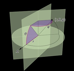
distance = f.sqrt(pointIndex+.2);
x = cos(longitude) * cos(latitude) * distance;
y = sin(longitude) * cos(latitude) * distance;
z = sin(latitude) * distance;

You might notice that rather than making distance a straight up function of the length pointIndex along the wire, I applied a square root. This is another one of those procedural tricks that seems arbitrary, but actually serves an important visual purpose. This is what the square root looks like (solid curve):

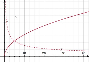
The dotted curve is the square root's derivative, i.e. it indicates the slope of the solid curve. Because the slope goes down with increasing distance, this trick has the effect of slowing down the outward motion of the wires the further they get. In practice, this means the wires are more tense in the middle, and more slack on the outside. It adds just enough faux-physics to make the effect visually appealing.

Rotation and Projection

Once I have absolute 3D coordinates for a point on a wire, I have to render it from the camera's point of view. This is done by moving the origin to the camera's position (X,Y,Z), and applying two rotations: one around the vertical (yaw) and one around the horizontal (pitch). It's like spinning on a wheely chair, while tilting your head up/down.

x -= X; y -= Y; z -= Z;

x2 = x * cos(yaw) + z * sin(yaw);
y2 = y;
z2 = z * cos(yaw) - x * sin(yaw);

x3 = x2;
y3 = y2 * cos(pitch) + z2 * sin(pitch);
z3 = z2 * cos(pitch) - y2 * sin(pitch);

The camera-relative coordinates are projected in perspective by dividing by Z — the further away an object, the smaller it is. Lines with negative Z are behind the camera and shouldn't be drawn. The width of the line is also scaled proportional to distance, and the first line segment of each wire is drawn thicker, so it looks like a plug of some kind:

plug = !pointIndex;
lineWidth = lineWidthFactor * (2 + plug) / z3;
x = x3 / z3;
y = y3 / z3;

lineTo(x, y);
if (z3 > 0.1) {
  if (lastPointVisible) {
    stroke();
  }
  else {
    lastPointVisible = true;
  }
}
else {
  lastPointVisible = false;
}
beginPath();
moveTo(x, y);

There's a subtle optimization hiding in plain sight here. Because I'm drawing lines, I need both the previous and the current point's coordinates at each step. To avoid using variables for these, I place the moveTo command at the end of the loop rather than at the beginning. As a result, the previous coordinates are remembered transparently into the next iteration, and all I need to do is make sure the first call to stroke() doesn't happen.

Coloring

Each line segment also needs an appropriate coloring. Again, I used some trial and error to find a simple formula that works well. It uses a sine wave to rotate overall luminance in and out of the (Red, Green, Blue) channels in a deliberately skewed fashion, and shifts the R component slowly over time. This results in a nice varied palette that isn't overly saturated.

pulse = max(0, sin(time * 6 - pointIndex / 8) - 0.95) * 70;
luminance = round(45 - pointIndex) * (1 + plug + pulse);
strokeStyle='rgb(' +
  round(luminance * (sin(plug + wireIndex + time * 0.15) + 1)) + ',' +
  round(luminance * (plug + sin(wireIndex - 1) + 1)) + ',' +
  round(luminance * (plug + sin(wireIndex - 1.3) + 1)) +
  ')';

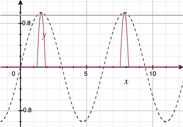
Here, pulse causes bright pulses to run across the wires. I start with a regular sine wave over the length of the wire, but truncate off everything but the last 5% of each crest to turn it into a sparse pulse train:

Camera Motion

With the main visual in place, almost all my code budget is gone, leaving very little room for the camera. I need a simple way to create consistent motion of the camera's X, Y and Z coordinates. So, I use a neat low-tech trick: repeated interpolation. It looks like this:

sample += (target - sample) * fraction

target is set to a random value. Then, every frame, sample is moved a certain fraction towards it (e.g. 0.1). This turns sample into a smoothed version of target. Technically, this is a one-pole low-pass filter.

This works even better when you apply it twice in a row, with an intermediate value being interpolated as well:

intermediate += (target - intermediate) * fraction
sample += (intermediate - sample) * fraction

A sample run with target being changed at random might look like this:

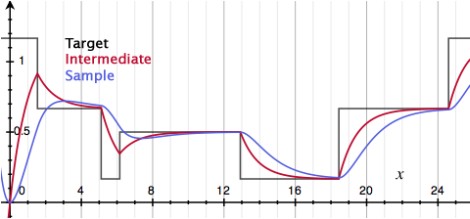
You can see that with each interpolation pass, more discontinuities get filtered out. First, jumps are turned into kinks. Then, those are smoothed out into nice bumps.

In my demo, this principle is applied separately to the camera's X, Y and Z positions. Every ~2.5 seconds a new target position is chosen:

if (frames++ > 70) {
  Xt = random() * 18 - 9;
  Yt = random() * 18 - 9;
  Zt = random() * 18 - 9;
  frames = 0;
}

function interpolate(a,b) {
  return a + (b-a) * 0.04;
}

Xi = interpolate(Xi, Xt);
Yi = interpolate(Yi, Yt);
Zi = interpolate(Zi, Zt);

X  = interpolate(X,  Xi);
Y  = interpolate(Y,  Yi);
Z  = interpolate(Z,  Zi);

The resulting path is completely smooth and feels quite dynamic.

Camera Rotation

The final piece is orienting the camera properly. The simplest solution would be to point the camera straight at the center of the object, by calculating the appropriate pitch and yaw directly off the camera's position (X,Y,Z):

yaw   = atan2(Z, -X);
pitch = atan2(Y, sqrt(X * X + Z * Z));

However, this gives the demo a very static, artificial appearance. What's better is making the camera point in the right direction, but with just enough freedom to pan around a bit.

Unfortunately, the 1K limit is unforgiving, and I don't have any space to waste on more 'magic' formulas or interpolations. So instead, I cheat by replacing the formulas above with:

yaw   = atan2(Z, -X * 2);
pitch = atan2(Y * 2, sqrt(X * X + Z * Z));

By multiplying X and Y by 2 strategically, the formula is 'wrong', but the error is limited to about 45 degrees and varies smoothly. Essentially, I gave the camera a lazy eye, and got the perfect dynamic motion with only 4 bytes extra!

Addendum

After seeing the other demos in the contest, I wasn't so sure about my entry, so I started working on a version 2. The main difference is the addition of glowy light beams around the object.

As you might suspect, I'm cheating massively here: rather than do physically correct light scattering calculations, I'm just using a 2D effect. Thankfully it comes out looking great.

Essentially, I take the rendered image, and process it in a second Canvas that is hidden. This new image is then layered on the original.

I take the image and repeatedly blend it with a zoomed out copy of itself. With every pass the number of copies doubles, and the zoom factor is squared every time. After 3 passes, the image has been smeared out into an 8 = 2³ 'tap' radial blur. I lock the zooming to the center of the 3D object. This makes the beams look like they're part of the 3D world rather than drawn on later.

For additional speed, the beam image is processed at half the resolution. As a side effect, the scaling down acts like a slight blur filter for the beams.

Unfortunately, this effect was not very compact, as it required a lot of drawing mode changes and context switches. I had no room for it in the source code.

So, I had to squeeze out some more room in the original. First, I simplified the various formulas to the bare minimum required for interesting visuals. I replaced the camera code with a much simpler one, and started aggressively shaving off every single byte I could find. Then I got creative, and ended up recreating the secondary canvas every frame just to avoid switching back its state to the default.

Eventually, after a lot of bit twiddling, a version came out that was 1024 bytes long. I had to do a lot of unholy things to get it to fit, but I think the end result is worth it ;).

Closing Thoughts

I've long been a fan of the demo scene, and fondly remember Second Reality in 1993 as my introduction to the genre. Since then, I've always looked at math as a tool to be mastered and wielded rather than subject matter to be absorbed.

With this blog post, I hope to inspire you to take the plunge and see where some simple formulas can take you.