Let's start where Isaac Newton supposedly did, with an apple.

Gravity kicks in. The apple bounces off the ground, losing some energy in the process. After a few bounces, its kinetic energy (speed) and potential energy (height) have both dissipated, and the apple is at rest.

But analyzing motion by watching it in real-time is tricky. It's better to visualize time as its own dimension, here horizontal, and look at the entire animation as a whole.

The apple's position $ \class{blue}{p(t)} $ moves through space and time, along arcs of decreasing height and duration. Once at rest, it continues advancing through time, without moving in space. In common parlance, this is the animation's easing curve.

It's worth pointing out they're not really arcs. This animation consists of individually numbered frames $ i $, switching 60 times per second. While a frame is displayed, the position $ \class{blue}{p_i} $ of the apple is constant. In between its value changes instantly, at times $ t_i $.

For convenience's sake, it's reasonable to consider this a curve, approximated by a series of straight lines. After all, that's the illusion that the animation successfully tricks us into seeing. The discrete nature of the curve will let us dissect it more easily. We're interested in the physics of this motion.

To determine the speed of the apple, we find the slope of a line segment: vertical divided by horizontal. Dividing distance by time gives us speed, e.g. meters per second. But actually, we're dealing with its cousin velocity which has a direction too. Positive slope means going up, negative slope means going down. This operation is called a forward or backward difference, depending on whether you look forward ($ \class{green}{v_{i→}} $) or backward ($ \class{green}{v_{←i}} $) around a point.

Forward differences tell us about what's happening between two adjacent points. We're more interested in what's happening at the points themselves. To fix this, we can take a central difference $ \class{green}{v_{i↓}} $, spanning two frames instead. We now get a good approximation for the slope directly at a point of interest, and thus the velocity.

If we apply this procedure along the entire curve, we can graph the apple's velocity over time, in sync with its position. This is the discrete version of taking the derivative in calculus, or differentiation and shows these two quantities are intimately related.

While in the air, the apple's velocity decreases along a straight line, first positive, then negative. On impact, the velocity suddenly reverses, though only to a portion of its previous value. At the top of each arc, the velocity passes through zero, which means the apple essentially hangs motionless in the air for a fraction of a second.

To further analyze this, we can repeat the procedure, and find the slope of the velocity. This is the change in velocity over time, better known as acceleration. It can be expressed in meters per second per second, that is, $ m / s^2 $. According to Newton, acceleration is force divided by mass: the heavier something is, the less effect the same force has.

What looked like a complicated animation at the position level is now revealed to be very simple: the apple undergoes a small constant acceleration downwards from gravity. It also experiences a short burst of much stronger acceleration upwards whenever it bounces. Once the upward force goes below a critical threshold, the apple stops moving. At the end, gravity is countered by the apple's resistance to being squished, and the net acceleration is zero.

Suppose we were given only the acceleration, and wanted to reconstruct the animation. Can we do that?

Yep, we just work our way back up. If the acceleration represents a difference in velocity over time, then we can track the velocity by adding these differences back, accumulating them one step at a time. Since we divided the differences by time initially, we'll now have to multiply each value by the time between frames. Technically we need forward differences ($ \class{orangered}{a_{i→}} $) for this, not central ones ($ \class{orangered}{a_{i↓}} $), but the error will be minor.

In calculus, this accumulation process is called integration. In our case, it's a sum ($ \sum $). As we are multiplying the vertical value $ \class{orangered}{a_{k→}} $ by the horizontal time step $ Δt $, each term represents the area of a thin rectangle. By adding up all these signed areas, positive for up and negative for down, we can approximate the integral and get velocity back. Integrals and areas under curves are very closely linked.

Similarly, we can integrate velocity into position by adding up strips of area under the velocity curve, recreating the original bounce. Note that for both sums, we needed to manually specify the starting point. If we didn't set it correctly, the apple would drift, bounce on thin air or penetrate the ground.

We've produced real physical behavior from raw forces like gravity. That means we've just described a real physics engine. It's a one-dimensional one, but a physics engine none the less. It implements Euler integration, a fast but generally inaccurate method. In this case, the reconstruction is not perfect due to the earlier mentioned usage of central rather than forward differences.

We only need one of the three in order to produce a plausible copy of the other two. That means we can control animations on any of the three levels. If we want full control, we specify position directly. For simple constrained motions, we can manipulate velocity and integrate once. For full-on physics, we set acceleration from physical laws and integrate twice. This is why the Newtonian model of motion is so important.

It also reveals smoothness. A smooth animation isn't just continuous in its path. Its velocity is continuous too, without sudden jumps. In some cases, we'll even want smooth acceleration too. An ordinary bounce effect is shown to involve a large acceleration, a sudden jerk. This is a noticeable visual disruption, the kind we generally want to avoid. If you've ever tried to ignore a bouncing icon, you'll know how hard this is.

In fact, jerk is what we call the slope of acceleration. That's three derivatives deep, and it's turtles all the way down. The next ones are imaginatively called snap, crackle and pop, though they signify little directly. A large jerk however implies a sudden, jarring change in force.

There's more physics hiding in plain sight. Earlier on, I mentioned energy: kinetic and potential. The apple's available potential energy $ \class{purple}{E_p} $ comes from gravity and is proportional to its height $ h $ above the ground, as well as the mass $ m $ and the local strength of gravity $ g $.

The kinetic energy $ \class{cyan}{E_k} $ comes from its motion. It's proportional to the velocity squared. That means each additional meter per second makes the previous ones more energetic, adding more kinetic energy the faster it's already going. To explain, we can imagine the force required to stop a moving object. By increasing the speed, you don't just add additional momentum: the impact also takes less time, concentrating it.

In a closed system, total momentum is conserved. As we are treating gravity as an outside force, this does not apply. Energy is conserved however. There's a vertical symmetry, where one energy level goes up as the other goes down, and vice versa. So we actually have a fourth level to control physics at: that of energy and potential. With some minor bookkeeping, we can create motion this way, called Hamiltonian mechanics.

The total energy, potential plus kinetic, is perfectly constant between bounces. On impact, a significant amount is lost. Note that the dips towards zero are a side effect of the finite approximation: if the bounce occurs between two frames, the apple appears to slow down for a frame, instantly falling down and bouncing back to where it was one frame earlier. Finite differences are oblivious to this.

The energy levels follow a decaying exponential curve. This is very typical: exponentials show up whenever a quantity is related to its rate of change. Hamiltonian models are useful for more complicated things like 3D roller coasters, where they allow you to abstract away complex interactions into a few concise relations like this.

In simple animation though, we'll generally stick to the direct Newtonian model. We can use it to analyze real use cases. Let's start with a common easing curve, cosine interpolation, used by default in jQuery.animate() and these slides too.

We animate the apple's position, changing its Y coordinate. In practice, that means we apply linear interpolation, lerping, between the start $ \class{orangered}{a} $ and end $ \class{green}{b} $. We take the starting point and add a fraction $ f $ of the difference $ \class{green}{b} - \class{orangered}{a} $ to it. Half the difference gets us halfway there, and so on. As long as $ f $ is between 0 and 1, we end up somewhere in the middle. When $ f $ reaches 1, the animation is complete.

The purpose of the easing curve is then to make the animation non-linear, not in space, but in time: in this case, the apple smoothly starts and stops. We can use any curve we like, e.g. half of a cosine wave of period 2. This eased lerp is the basic building block of any animation system.

The effect of the easing curve is visible when we take central differences again, and look at velocity and acceleration. The acceleration has been divided by 3 to fit. This doesn't seem bad, all three quantities appear to change smoothly. This picture is deceptive though.

All curves continue before and after the animation. The smooth cosine ease turns out to be quite jarring in its acceleration: it's like flooring the accelerator from standstill then easing off gently. At the halfway point you start braking, more and more until you stop. It's one of the most responsive animations possible that's still smooth at both ends. Smoother easing curves have smoother accelerations, but respond slower.

A simpler example is the half-ease, here achieved with a quadratic curve $ \class{blue}{f^2} $. The velocity is a linearly increasing ramp. The acceleration is constant, except for a very large instant deceleration at the end. This is like flooring the accelerator from standstill, holding it down for the duration, and then crashing into a wall—the suicide ease. Due to this, half-easing is typically used for fading transitions, where the object is invisible–or the audio inaudible–at the start or end.

But we can repurpose it quite easily. By tweaking this at the velocity level, we can maintain a constant speed at the end. This is the slow start, and can be expressed directly as an open-ended easing curve. In this case, we allow $ f $ to exceed 1, and the linear interpolation turns into extrapolation for free, no extra charge. We can scale the curve vertically to change the final speed, and scale it horizontally to control the delay. The slow start (and stop) is used throughout these slides.

We can combine curves too. Here, we add a cosine wave to the slow start, creating perhaps the motion of a rising jellyfish. Adding up animations is an easy way to create variations on a theme, used often in the demoscene. The derivatives add straight up too, so all three curves shift up and down by a sine or cosine wave. You can see how a small shift in position can have a large effect on both velocity and acceleration.

The next example is a bit different. Any guesses as to what this is? The hint is in the vertical scale, now measured in pixels. This animation moves almost 1000 pixels in just over one second.

It's an inertial flick gesture, recorded on Mac OS X. We can plot velocity and acceleration again. There's a slight measurement error, visible as noisy ripples on the acceleration, even after smoothing out the data: derivatives are very sensitive to noise. The velocity and acceleration have also been scaled down to fit, as they are both quite large.

The first part of the curve is not an animation at all: it was tracking the direct motion of my finger. Fingers move very smoothly: the acceleration follows a curve up and down. This is more physics: of nerve signals causing muscle fibers to contract and digits to move. This work smoothly converts chemical potential into kinetic energy. The small jump in speed at time 0 is easy to explain: my finger was already moving when it touched the pad.

The second part is the actual inertial animation. It kicks in as soon as the finger leaves the pad. All three values follow an exponential curve past that point, disregarding the noise. But the important one is velocity: the animation starts with the last known velocity and smoothly decays it to zero. Where we end up depends on how fast we were going when the finger left the pad.

Inertial scroll is easiest to control at the velocity level. We can measure the initial velocity by finding the position's slope, usually averaged over several frames. We then start at this velocity, but reduce it every frame by a fraction $ \class{royal}{f} $, which is a coefficient of friction. We don't need to care how far we'll go or how long it'll take: we can just keep animating until the velocity gets close enough to 0.

Suppose we do care where we end up. We might be showing a list of items, each 100 pixels tall. It could be good to control the animation so it always stops right at an item. We can't violate the principle of smooth motion, so we can't just change the position or velocity directly. We have to change the coefficient of friction.

As the velocity follows a simple curve, we don't have to track it manually. We can express it over time as a direct relation, based on the initial velocity $ \class{green}{v_{0→}} $. The exponential nature is clear, with the frame number $ i $ appearing as the exponent of a number between 0 and 1.

The position at frame $ i $ is then the sum of all the previous velocities times the time step $ Δt $, just like before, relative to the initial position $ \class{blue}{p_0} $. As the time step and initial velocity are constant, we can move both outside the sum.

To find the final resting position, we theoretically have to continue the animation all the way to infinity. This can be done using a limit. For now, we'll just look up the formula for this infinite sum, a geometric series. We end up dividing by the coefficient of friction: the lower it is, the further we go after all. If the coefficient were 0, there'd be no friction. We'd divide by zero, because there's no final resting position when you never slow down.

We can invert this relationship to find the coefficient of friction required to stop at a given target. We just need the initial distance to the target, $ \class{blue}{Δp} $. To apply this in practice, we determine the friction needed to reach the next couple of items, and pick the one which is closest to the default case. The user won't notice the subtle change in friction—the UI will just magically seem better.

The simulation works identical in all cases and the velocities are still continuous and exponential, which means: physical. This effect only requires one additional calculation at the start, which makes it all the more strange that developers have come up with increasingly jarring ways to achieve something similar.

Now let's try animating in 2D.

We can move the apple in 2D by animating its X and Y coordinates. Here we animate both in lockstep, using a sine wave: the apple moves diagonally, as X and Y are always equal. By adjusting their relative amplitudes, we can control the angle of motion.

If we animate X and Y separately, we create arbitrary paths. Here they both follow a sine wave, but with different frequencies. The resulting path is called a Lissajous curve. The sine waves drift in and out of phase, going from a diagonal to an oval to a circle, and back again.

It makes more sense to picture the position as a 2D vector, an arrow. It has both a direction and a length, relative to the origin. While the calculation is equivalent—animating X and Y separately—the vector representation is more natural once we look at the derivatives.

What does slope and velocity mean in this context? The same principle applies: we take the difference in position between two frames, and divide it by the difference in time $ Δt $. In this case, all quantities except time are vectors.

As a single frame is very short, the velocity is quite large, and always tangent to the path. Its length directly represents speed.

If we center the velocity vector, it traces out its own Lissajous curve. This one is slightly different and doubles back on itself at regular intervals.

We can apply finite differences again to dissect velocity into acceleration. It follows yet another Lissajous curve, a scaled and rotated version of the position.

Finally, we can disentangle these curves by plotting them out over time. Position, velocity and acceleration dance around each other. Despite its artificial construction, even this motion is physical: it's what happens when you take an object and hang it off independently moving horizontal and vertical springs of different stiffness. With the right visualization, raw physics is quite beautiful in its own right.

So far, we've assumed a constant frame rate.

If our animation is defined by an easing curve, we can look up its value at any point along the way.

It seems at first, variable frame rates are trivial: we can evaluate the curve at arbitrary times instead of pre-set intervals.

If we take forward differences to measure slope, we still get a smooth velocity curve. We can accumulate—integrate—these differences back into position as long as we account for a variable time step $ Δt_i $. It seems our physics engine should be unbothered too. But there's a few problems.

First, if we implemented inertial scrolling like we did before, multiplying the velocity by $ 1 - \class{royal}{f} $ every frame, we'd get the wrong curve. The amount of velocity lost per frame should now vary, we can no longer treat it as a convenient constant.

If we do the math, we can find an expression for the correct amount of friction $ \class{purple}{f_i} $ per frame for a given step $ Δt_i $, relative to the default $ \class{royal}{f} $ and $ Δt $. Not pretty, and this is just one object experiencing one force. In more elaborate scenarios, finding exact expressions for positions or velocities can be hard or even impossible. This is what the physics engine is supposed to be doing for us.

There's another problem. If we integrate these curve segments to get position, we get an exponential curve, just as before. Did we achieve frame rate independence?

Well, no. If we change the time steps and run the algorithm again, it looks the same. However, the new curve and old curve don't match up. The difference is surprisingly large, as this animation is only half a second long and the average frame rate is identical in both cases. Such errors will compound the longer it runs, and make your program unpredictable.

Luckily we can have our cake and eat it too. We can achieve consistent physics and still render at arbitrary frame rates. We just have to decouple the physics clock from the rendering clock.

Whenever we have to render a new frame, we compare both clocks. If the render clock has advanced past the physics clock, we do one or more simulation steps to catch up. Then we interpolate linearly between the last two values until we run out of physics again.

This means the visuals are delayed by one physics frame, but this is usually acceptable. We can even run our physics at half the frame rate or less to conserve power. Though more error will creep in, this error will be identical between all runs, and we can manually compensate for it if needed.

When we implement variable frame rates correctly, we can produce an arbitrary number of frames at arbitrary times. This buys us something very important, not for the end-user, but for the developer: the ability to skip to any point in time, or at least fast-forward as quickly as your computer can manage.

But just because the simulation is consistent, doesn't mean it's correct or even stable. Euler integration fits our intuitive model of how pieces add up, but it's actually quite terrible. For example, if we made our bouncing apple perfectly elastic in the physical sense—losing no energy at all—and apply Euler, it would start bouncing irregularly, gaining height.

Which means the first bounce simulation wasn't using Euler at all. It couldn't have: the energy wouldn't have been conserved. All the finite differentiation and integration magic that followed only worked neatly because the position data was of a higher quality to begin with. We have to find the source of this phantom energy so we can correct for it, creating the Verlet integration that was used.

We're trying to simulate this path, the ideal curve we'd get if we could integrate with infinitely small steps. We imagine we start at the point in the middle, and would like to step forward by a large amount. The time step is exactly 1 second, so we can visually add accelerations and velocities like vectors, without having to scale them. Note that this is not a gravity arc, the downward force now varies.

Earlier, I said that if we used forward differences, we could get the velocity between two points. And that we could make a reconstruction of position from forward velocity by applying 'Euler integration'. While that's true, that's not actually what Euler integration is.

See, this is a chicken and egg problem. This velocity isn't the slope at the start or the end or even the middle. It's the average velocity over the entire time step. We can't get this velocity without knowing the future position, and we can't get there without knowing the average velocity in the first place.

The velocity that we're actually tracking is for the point itself, at the start of the frame. Any force or acceleration is calculated based on that single instant. If we integrate, we move forward along the curve's tangent, not the curve itself. This is where the extra height comes from, and thus, phantom gravitational energy.

For any finite step, there will always be some overshooting, because we don't yet know what happens along the way. Euler actually made the same mistake we made earlier: he used a central difference where a forward one was required, because the forward difference can only be gotten after the fact. The 'central difference' here is the actual velocity at a point, the true derivative.

As the acceleration changes in this particular scenario, we could try applying Euler, and then averaging the start and end velocities to get something in the middle. It fails, because the end velocity itself is totally wrong. Though we get closer than Euler did, we now undershoot by half the previous amount.

To resolve the chicken and egg, we need to look to the past. We assume that rather than starting with one position, we start with two known good frames, defined by us. That means we can take a backwards difference and now know the average velocity of the previous frame. How does this help?

Well, we assume that this velocity happens to be equal or close to the velocity at the halfway point. We also still assume the acceleration is constant for the entire duration. If we then integrate from here to the next halfway point, something magical happens.

We get a perfect prediction for the next frame's average velocity, the forward difference. By always remembering the previous position, we can repeat this indefinitely. That this works at all is amazing: we're applying the exact same operation as before—constant acceleration—for the same amount of time. On just a slightly different concept of velocity. Without even knowing exactly when the object reaches that velocity. That's Verlet integration.

Euler integration failed on a simple constant acceleration like gravity and can only accurately replicate a linear ease $ f $. This motion is a cubic ease $ f^3 $, with linear acceleration that decreases. Verlet still nails it, even when leaping seconds at a time. Why does this work?

Euler integration applies a constant acceleration ahead of a point. If there's any decrease in acceleration, it overestimates by a significant amount. That's on top of stepping in the wrong direction to begin with. Both position and velocity will instantly begin to drift away from their true values.

Verlet integration applies the same constant acceleration around a point. If the acceleration is a perfect line, the error cancels out: the two triangles make up an equal positive and negative area. By starting with a known good initial velocity and cancelling out subsequent errors, we can precisely track velocity through a linear force. If we simplify the formula, velocity even disappears: we can work with positions and acceleration directly.

As this captures the slope of acceleration, we only get errors if the acceleration curves. In this case, the left and right areas don't cancel out exactly. The missing area however smoothly approaches 0 as the time step shrinks, a further sign of Verlet's error-defeating properties. If we do the math, we find the position has $ O(Δt^2) $ global error: decrease the time step $ Δt $ by a factor of 10, and it becomes 100× more accurate. Not bad.

For completeness, here's the 4th order Runge-Kutta method (RK4), which is a sophisticated modification of Euler integration. It involves taking full and half-frame steps and backtracking. It finds 4 estimates for the velocity based on the acceleration at the start, middle and end.

The physics can then be integrated from a weighted sum of these estimates, with coefficients $ [\frac{1}{6}, \frac{2}{6}, \frac{2}{6}, \frac{1}{6}] $. We end up in the right place, at the right speed. This method offers an $ O(Δt^4) $ global error. Decrease the time step 10× and it becomes 10,000× more accurate. We have a choice of easy-and-good-enough (Verlet) or complicated-but-precise (RK4), at any frame rate. Each has its own perks, but Verlet is most attractive for games.

With physics under our belt, let's move on. Why not animate time itself? This is the variable speed clock and it's dead simple. It's also a great debugging tool: sync all your animations to a global clock and you can activate bullet time at will. You can tell right away if a glitch was an animation bug or a performance hiccup. On this site too: if you hold Shift, everything slows down 5×.

First, we differentiate the clock's time backwards—because in real-time applications, we don't know what the future holds. This is time's velocity $ \class{green}{v_{←i}} $. As we have to divide by the time step too, the velocity is constant and equal to 1. Let's change that.

We can reduce the speed of time at will, by changing $ \class{green}{v_i} $. If we then multiply by the time step $ Δt_i $ again and add the pieces back together incrementally, we get a new clock $ t'_i $. By integrating this way, we only need to worry about slope, not position: time always advances consistently. This is also where variable frame rates pay off: going half the speed is the same job as rendering at twice the frame rate.

Using our other tricks, we can animate $ \class{green}{v_i} $ smoothly, easing in and out of slow motion, or speeding into fast-forward. If we didn't do this, then any animation cued off this clock would jerk at the transition point. This is the chain rule for derivatives in action: derivatives compound when you compose functions. Any jerks caused along the way will be visible in the end result.

If time is smooth, what about interruptions? Suppose we have a cosine eased animation. After half a second, the user interrupts and triggers a new animation. If we abort the animation and start a new one, we create a huge jerk. The object stops instantly and then slowly starts moving again.

One way to solve this is to layer on another animation: one that blends between the two easing curves in the middle. Here it's just another cosine ease, interpolating in the vertical direction, between two changing values. We blend across the entire animation for maximum smoothness. This has a downside though: if the blended animation itself is interrupted, we'd have to layer on another blend, one for each additional interruption. That's too much bookkeeping, particularly when using long animations.

We can fix this by mimicking inertial scrolling. We treat everything that came before as a black box, and assume nothing happens afterwards. We only look at one thing: velocity at the time of interruption.

After determining the velocity of any running animations, we can construct a ramp to match. We start from 0 to create a relative animation.

We can bend this ramp back to zero with another cosine ease, interpolating vertically. This time however, the first easing curve is no longer involved.

If we then add this to the second animation, it perfectly fills the gap at the corner. We only need to track two animations at a time: the currently active one, and a corrective bend. If we get interrupted again, we measure the combined velocity, and construct a new bend that lets us forget everything that came before.

By using a different easing curve for the correction, we can make it tighter, creating a slight wave at the end. Either way, it doesn't matter how the object was moving before, it will always recover correctly.

But what if we get interrupted all the time? We could be tracking a moving pointer, following a changing audio volume, or just have a fidgety user in the chair. We'd like to smooth out this data. The interrupted easing approach would be constantly missing its target, because there is never time for the value to settle. There is an easier way.

We use an exponential decay, just like with inertial scrolling. Only now we manipulate the position $ p_{i} $ directly: we move it a certain constant fraction towards the target $ \class{purple}{o_{i}} $, chasing it. Here, $ \class{royal}{f} = 0.1 = 10\% $. This is a one-line feedback system that will keep trying to reach its target, no matter how or when it changes. When the target is constant, the position follows an exponential arc up or down.

The entire path is continuous, but not smooth. That's fixable: we can apply exponential decay again. This creates two linked pairs, each chasing the next, from $ \class{slate}{q_{i}} $ to $ \class{blue}{p_{i}} $ to $ \class{purple}{o_{i}} $. Each level appears to do something akin to integration: it smooths out discontinuities, one derivative at a time. Where a curve crosses its parent, it has a local maximum or minimum. These are signs that calculus is hiding somewhere.

That's not so surprising when you know these are difference equations: they describe a relation between a quantity and how it's changing from one to step to the next. These are the finite versions of differential equations from calculus. They can describe sophisticated behavior with remarkably few operations. Here I added a third feedback layer. The path gets smoother, but also lags more behind the target.

If we increase $ f $ to 0.25, the curves respond more quickly. Exponential decays are directly tuneable, and great for whiplash-like motions. The more levels, the more inertia, and the longer it takes to turn.

We can also pick a different $ f_i $ for each stage. Remarkably, the order of the $ \class{royal}{f_i} $ values doesn't matter: 0.1, 0.2, 0.3 has the exact same result as 0.3, 0.2, 0.1. That's because these filters are all linear, time-invariant systems, which have some very interesting properties.

If you shift or scale up/down a particular input signal, you'll get the exact same output back, just shifted and scaled in the same way. Even if you shift by less than a frame. We've created filters which manipulate the frequencies of signals directly. These are 1/2/3-pole low-pass filters that only allow slow changes. That's why this picture looks exactly like sampling continuous curves: the continuous and discrete are connected.

Exponential decays retain all their useful properties in 2D and 3D too. Unlike splines such as Bezier curves, they require no set up or garbage collection: just one variable per coordinate per level, no matter how long it runs. It works equally well for adding a tiny bit of mouse smoothing, or for creating grand, sweeping arcs. You can also use it to smooth existing curves, for example after randomly distorting them.

However there's one area where decay is constantly used where it really shouldn't be: download meters and load gauges. Suppose we start downloading a file. The speed is relatively constant, but noisy. After 1 second, it drops by 50%. This isn't all that uncommon. Many internet connections are traffic shaped, allowing short initial bursts to help with video streaming for example.

Often developers apply slow exponential easing to try and get a stable reading. As you need to smooth quite a lot to get rid of all the noise, you end up with a long decaying tail. This gives a completely wrong impression, making it seem like the speed is still dropping, when it's actually been steady for several seconds. The same shape appears in Unix load meters: it's a lie.

If we apply double exponential easing, we can increase $ f $ to get a shorter tail for the same amount of smoothing. But we can't get rid of it entirely: the more levels of easing we add, the more the curve starts to lag behind the data. We can do much better.

We can analyze the filters by examining their response to a standard input. If we pass in a single step from 0 to 1, we get the step response for the two filters.

Another good test pattern is a single one frame pulse. This is the impulse response for both filters. The impulse responses go on forever, decaying to 0, but never reaching it. This shows these filters effectively compute a weighted average of every single value they've ever seen before: they have a memory, an infinite impulse response (IIR).

Doesn't this look somewhat familiar? It turns out, the step response is the integral of the impulse response. It's a position. Vice versa, the impulse response is the derivative of the step response. It's a velocity. Surprise, physics!

But it gets weirder. Integration sums together all values starting from a certain point, multiplied by the (constant) time step. That means that integration is itself a filter: its impulse response is a single step, the integral of an impulse. Its step response is a ramp, a constant increase.

It works the other way too. Differentiation takes the difference of neighbouring values. It's a filter and its step response is just an impulse, detecting the single change in the step. Its impulse response is an upward impulse followed by a downward one: the derivative of an impulse. When one value is weighed positively and the other weighed negatively, the sum is their difference.

This explains why exponential filters seem to have integration-like qualities: these are all integrators, they just apply different weights to the values they add up. Every step response is another filter's impulse response, and vice versa, connected through integration and differentiation. We can use this to design filters to spec.

That said, filter design is still an art. IIR filters are feedback systems: once a value enters, it never leaves, bouncing around forever. Controlling it precisely is difficult under real world conditions, with finite arithmetic and noisy measurements to deal with. Much simpler is the finite impulse response (FIR), where each value only affects the output for a limited time. Here I use one lobe of a sine wave over 4 seconds.

Even if we don't know how to build the filter, we can still analyze it. We can integrate the impulse response to get the step response. But there's a problem: it overshoots, and not by a little. Ideally the filtered signal should settle at the original height. The problem is that the area under the green curve does not add up to 1.

To fix this, we divide the impulse response by the area it spans, $ \class{green}{\frac{8}{π}} $, or multiply by $ \class{green}{\frac{π}{8}} $, normalizing it to 1. Such filters are said to have unit DC gain, revealing their ancestry in analog electronics. The step response turns out to be a cosine curve, and this filter must therefore act like perpetually interruptible cosine easing.

There's two ways of interpreting the step response. One is that we pushed a step through the filter. Another is that we pushed the filter through a step—an integrator. This symmetry is a property of convolution, which is the integration-like operator we've been secretly using all along.

Convolution is easiest to understand in motion. When you convolve two curves $ \class{purple}{q_i} ⊗ \class{green}{r_i} $, you slide them past each other, after mirroring one of them. As our impulse response is symmetrical, we can ignore that last part for now.

We multiply both curves with each other, creating a new curve in the overlap: here a growing section of the impulse response. The area under this curve is the output of the filter at that time. The sum goes to infinity in both directions, allowing for infinite tails. We already saw something similar when we used a geometric series to determine the final resting position of an inertial scroll gesture. With a FIR filter, the sum ends.

But why did we have to mirror one curve? It's simple: from the impulse response's point of view, new values approach from the positive X side, now left, not the negative X side, right. By flipping the impulse response, it faces the other signal, which is what we want.

If we center the view on the impulse response, it's clear we've swapped the role of the two curves. Now it's the step that's passing backwards through the filter, rather than the other way around.

If we replace the step response with a random burst of signal, the filter can work its magic, smoothing out the input through convolution. It's a weighted average with a sliding window. The filter still lags behind the data, but the tail is now finite.

If we make the window narrower, its amplitude increases due to the normalization. We get a more variable curve, but also a shorter tail. This is like a blur filter in Photoshop, only in 1D instead of 2D. As Photoshop has the entire image at its disposal, rather than processing a real-time signal, it doesn't have to worry about lag: it can compensate directly by shifting the result back a constant distance when it's done.

What about custom filter design? Well, if you're an engineer, that's a topic for advanced study, learning to control the level and phase at exact frequencies. If you're an animator, it's much simpler: you pick a desired easing curve, and use its velocity to make a normalized filter. You end up with the exact same step response, turning the easing curve into a perpetually interruptible animation.

Which leads to the last trick in this chapter: removing lag on a real-time filtered signal. There's always an inherent delay in any filter, where signals are shifted by roughly half the window length. We can't get rid of it, only reduce it. We have to change the filter to prefer certain frequencies over others, making it resonate to the kind of signal we expect. We use an easing curve that overshoots, and preferably a short one. This is just one I made up.

The velocity—here scaled down—now has a positive and negative part. As neither part is normalized by itself, the filter will first amplify any signal it encounters. The second part then compensates by pulling the level back down.

The result is that the filter actually tries to predict the signal, which you can imagine is a useful thing to do. At certain points, the lag is close to 0, when the resonance frequency matches and slides into phase. When applied to animation, resonant filters can create jelly-like motions. When applied to electronic music at about 220 Hz, you get Acid House.

Let's put it all together, just for fun. Here we have some particles being simulated with Verlet integration. Each particle experiences three forces. Radial containment pushes them to within a certain distance of the target. Friction slows them down, opposing the direction of motion. A constantly rotating force, different for each particle, keeps them from bunching up. The target follows the mouse, with double exponential easing.

Friction links acceleration to velocity. Containment links acceleration to position. And integration links them back the other way. These circular dependencies are not a problem for a good physics engine. Note that the particles do not interact, they just happen to follow similar rules.
Tip: Move the mouse and hold Shift to see variable frame rate physics in action.

If we add up the three forces and trace out curves again, we can watch the particles—and their derivatives—speed through time. Just like you are doing right now, in your chair. As velocity and acceleration only update in steps, their curves will only be smooth if the physics clock and rendering clock are synced.

This a classic keyframe timeline: a set of frames, with values defined along the way. It could be a vertical or horizontal motion, the opacity of a shape, the volume of a sound, etc. Any one thing we want to animate precisely over a long time.

This is one second of a 60 fps animation and there's a keyframe every 10 frames. We can interpolate between the points with a cosine ease. But there's already a mistake.

By expressing animations as frames, we can only have animations that are multiples of the frame length. In this case, that's 16.6 ms. If we want to space keyframes at 125ms, we can't, because that's 7.5 frames. The closest we can manage is alternating 7 and 8 frame sections.

Just like with variable frame rates, we need to set keyframes in absolute time, not numbered frames. We use a global clock to produce arbitrary in-between frames. If we change our mind and wish to speed up or slow down part of our timeline, there's no snap-to-frame to get in our way. Note that Adobe Flash does not do this: you define your frame rate up front and are stuck with it.

There is a catch though, easy to overlook: by the time we notice the first animation has ended, the second one has already started. We need to account for this slack, and make sure we start partway in, not from the beginning. Otherwise, this error accumulates with every keyframe, leading to noticeable lag.

This is also important for triggered actions like sound. Suppose there is a performance glitch right before it plays, and we lose 7 frames. Rare, but not impossible. If we don't account for slack, we'd have 7.5 frames of permanent lag on the audio, 125ms. More than enough to disrupt lip sync. Instead we should skip ahead to make up for it. To avoid an audible pop when skipping audio, we can apply a tiny fade in: a microramp.

With real-time dependencies like audio, it's better to be safe than sorry though. As the audio subsystem is generally independent, we can avoid this issue by pre-queuing all the sound with a delay. Here we begin playback 100ms earlier, but start each sound with an implied 100ms silence, minus the slack. Now, no audio will be lost in most situations. This too is animation: micromanaging time.

Let's focus our attention back on this easing curve. By treating it as a sequence of individual animations, we've created a smooth path. But it's not a very ideal path: it stops at every keyframe and then starts moving again, creating a curve with stairs. This is more obvious if we plot the velocity.

We need to replace it with a spline, a designable curve. There's too many to name, but we'll stick to a common one: Catmull-Rom splines. It's entirely based on one particular curve. Looks suspiciously like an impulse response, doesn't it?

But actually, it's not one curve, it's 4 separate cubic curves glued together into a symmetric pulse. They're designed so their velocities meet up at the transition, thus creating a single smooth path. But if you look closely, you can see that the velocity (scaled) has two minor kinks in it, one on each side.

There are two other important features. The first is that the curve goes through 0 at all the keyframes except the central one. There, its value is 1. The keyframes are called the knots of the spline.

The other is that its slope is 0 at all the knots except the ones adjacent to the peak. There, it's $ \frac{1}{2} $ and $ -\frac{1}{2} $ respectively. If we trace the slopes out to the center, we go half as high as the peak, to 0.5.

That means if we scale down this curve as a whole, very few things we're interested in actually change. All the horizontal slopes remain horizontal. All the knots at 0 remain at 0. Only the peak shrinks, and the slopes at the adjacent knots go down.

We can literally treat the curve as the impulse response of a filter, and the knots as a series of impulses. A filter outputs a copy of its impulse response for every impulse it encounters. As this is all theoretical, we don't care about filter lag.

If we now add up all the curves, we get the Catmull-Rom spline. Despite the intricate interactions of the curves between the knots, the result is very predictable. The spline goes through every keyframe, because the values at the knots are all 0 except for the peak itself.

What's more, when we move a single value up and down, only two other things change: the two slopes at the adjacent knots. The slope at the knot itself is still constant. This means we can control the initial and final slope of the spline just by adding an extra knot before and after: it won't affect anything else.

See, the slope at a knot is actually just the central difference around that point. This is where the factor of $ \frac{1}{2} $ for the adjacent slopes came from earlier, and why their signs were opposite: it's a difference that spans two keyframes, so we divide by 2. This is the rule that determines how Catmull-Rom splines curve.

There's just one problem: all of this only works if the keyframes are equally spaced. If we change the spacing, our base curve is no longer smooth: there is a kink at the adjacent keyframes. This might not look like much, but it would be noticeable.

There's two ways to solve this. One is to try and come up with a unique curve for every knot. This curve has to be smooth and hit all the right values and slopes. This is the hard way, and can result in odd changes of curvature if done badly, like here.

But actually, you already know the other solution. By distorting the Catmull-Rom spline to fit our keyframes, it's like we've rendered it with a variable speed clock. But one that doesn't change smoothly. This is why the curves have developed kinks out of nowhere. If we can smooth out the passage of time, then we'll stretch the spline smoothly between the keyframes.

We can just create another Catmull-Rom spline to do so. Horizontally, we put equally spaced knots. This dimension has no real meaning: it's just 'spline time' now, independent of real time.

We move the knots vertically to the keyframe time and make a spline. In this case, I tweaked the start and end to be a diagonal rather than a horizontal slope. This curve hits all the keyframes at the right time and transitions smoothly between them. It's a variable clock that goes from constant spline time to variable real time.

To actually calculate the animation, we need to go the other way and invert the relationship: from variable real time to constant spline time. This can be done a few ways, but the easiest is to use a binary search, as the time curve always rises: it's like finding a value in an ordered list. This tells us how fast to scrub through the spline.

With this, we can warp the Catmull-Rom spline to hit all the keyframes at the right times. We'll still need to manually edit the keyframes to get a perfectly ripple-free path, but now we can move them anywhere, anytime we like.

What we just did was to chart a path through 1D space and 1D time, by combining two Catmull-Rom splines. Add time travel, and this is entirely equivalent to charting a random 2D spline through 2D space. To create such an animation, you create two parallel tracks, one for X and one for Y, with identical timings. By scrubbing through spline time, you move in both X and Y, and hence along the curve. However, doing so precisely turns out to be complicated.

In the 1D case, the distance between two keyframes is trivial: going from 0 to 1 means you moved 1 unit. In the 2D case, that's no longer true: the distance travelled depends on both X and Y simultaneously. What's worse is, splines generate uneven paths. If we divide them equally in spline time, we get unequal steps in real time. The apple slows down and then shoots off.

It might seem cool that the spline naturally has a tension in its motion, but it will only get in the way. If we move just a single X coordinate of a single knot, the entire path shifts, and the distance between the steps changes considerably. The easing of the Y coordinate needs to compensate for this. We can't maintain a controlled velocity this way: X and Y are dependent and have to be animated together.

We can resolve this by doing for distance what we did for time: we have to make a map from spline time to real distance. We can step along the spline in small steps and measure the distance one line segment at a time. When we integrate, adding up the pieces, we get a curve that maps spline time onto total distance along the curve.

Again, we can invert the relationship to get a map from distance to spline time.

We can use it to divide the spline into segments of equal length and move an object along the path with a constant speed. This works for any spline, not just Catmull-Rom. We can always turn a curve into a neat set of equally spaced points of our choosing.

The distance map gives us a natural parametrization: a way to move along the curve by the arc length itself. This effectively flattens out the curve into a straight line, and we can treat it like a 1D animation. We can apply straightforward easing again, because distances are once again preserved.

To animate, we just define an easing curve for distance over time. If we want to move along the path at a constant speed, we line the keyframes up along a diagonal.

However, the knots don't have any special meaning anymore. When we move, we pass through them at just the same speed as any other point. That means we can control velocity completely independent of the path itself, using all the tricks from earlier. We can also apply a direct easing curve along the path, for example cubic easing.

To run the animation, we go the other way. The easing curve tells us the desired distance along the path at any moment in time. We have to use the inverse distance map to convert this to spline time for the point in question.

Then we can use the spline time to look up the point on the Catmull-Rom spline. The easing curve makes us scrub smoothly along the distance map. This in turn makes us move smoothly on the spline—albeit with a bit of whiplash.

While that might seem like a lot of work, the good news is, it works in 3D too. We can find a distance map based on 3D distance, and now have three simultaneous Catmull-Rom splines for the X, Y and Z coordinates.

In a way, path-based animation is cheating: it acts like there's an infinitely strong force keeping the object on the track, only we don't need physics to make it happen. If we did add other forces however, we'd get a miniature WipeOut-style racing game. This principle is applied in the demo at the top of this page: the velocity along the track is constant, but the camera and its target are being exponentially eased, creating lag and swings in corners, giving it a natural feel.

What's wrong with angles? Let's ask our trusty friend, the apple. Sorry, I got hungry.

Well, they wrap around. Suppose we have an object that's been rotated a couple of times, for example as part of an interactive display. It completed 2.3 turns ($ τ = 2π $) around the circle. For now we'll use degrees, but eventually we'll switch to radians for the heavier stuff.

If we animate the apple to a target angle $ \class{purple}{\phi_T} $ at 0°, it will spin all the way back. Our animation system doesn't know that it could stop earlier at 720° or 360°.

To fix this, we can't simply reduce all angles to the interval 0…360. If we animate from 0 to 315°, we still go the long way around rather than just 45° in the other direction.

We need to reduce the difference in angle $ \class{purple}{\phi_T} - \class{blue}{\phi} $ to less than 180° in either direction. This is a circular difference, easiest when counting whole turns $ δ $, so we can round off to $├\,δ\,┤$. The difference, e.g. $ 3.3 - 3 = 0.3 $ or $ 1.6 - 2 = -0.4 $ is never more than half a turn. If we now set the target to 90°, it tells us to animate by $ \class{green}{+135°} $, that is, the short way around.

Our angles are now still continuous, going beyond 360° in either direction, but we never rotate more than 180° at a time unless we actually want to. We can apply this correction whenever we interpolate between two angles, and always end up at an equivalent angle.

Here I use double exponential easing to chase a rapidly changing angle. The once filtered angle jerks whenever it gets lapped, as it suddenly needs to change direction. The twice filtered angle moves smoothly however.

What about 3D? If we're restricting ourselves to a single axis of rotation, nothing really changes. We still control the angle the same way.

But orientation in 3D is a complicated thing. The easiest way to express it is with a 3×3 matrix: this is a set of 3 vectors in 3D. They define a frame of reference in space, a basis: right/left, up/down and forward/back. When we rotate around the vertical axis $ \vec y $, we rotate $ \vec x $ and $ \vec z $ together.

For arbitrary orientations, $ \vec x $, $ \vec y $ and $ \vec z $ can turn in any direction, but always maintain a perfect 90° angle between themselves.

Each vector is a set of $ (x, y, z) $ coordinates. That means we can write down the matrix as a set of 3 triples of coordinates, one column for each vector. At first it would seem we need 9 numbers to describe a 3D rotation. We can apply this rotation matrix to transform any point $ (x, y, z) $ by adding up proportional amounts of $ \vec x $, $ \vec y $ and $ \vec z $. This is linear algebra.

But there's tons of redundancy here. Because the 3 vectors are perpendicular, $ \vec z $ can only be in one of two places. The difference between the two is called a left handed or right handed coordinate system: for thumb, index and middle finger, with your hand shaped like a gun and the middle finger sticking out.

So long as we agree on a common style of coordinate system, for example right-handed, we don't need to track $ \vec z $. We can recover it from $ \vec x $ and $ \vec y $ using something called the vector cross product. The vector that comes out will always be perpendicular to the two we pass in, decided by a left- or right-hand rule. This is by the way how you can aim a camera in 3D: all you need is a target, and an up vector.

We're down to 6 numbers. But there's more. A rotation preserves length, so the basis must always stay the same size. All the vectors must have length 1—be normalized—and hence move on the surface of a sphere.

Instead of 3 coordinates, we can remember $ \vec x $ as two angles: longitude $ \phi $ and latitude $ \theta $. First we rotate around the Y axis, then around the rotated Z axis. Did we uniquely determine $ \vec y $ as well?

No, there is a third degree of freedom we haven't been using so far. In order to account for all the places where $ \vec y $ can be, we need to allow rotation around $ \vec x $, by another angle $ \gamma $. Now we can describe any orientation in 3D using just three numbers, the so called Euler angles.

This is a YZX gyroscope, after the order of rotations used. We can build one in real life by using concentric rings connected by axles. Make one large enough to put a chair in the middle, and you've got an amusement ride—or something to train pilots with. When we rotate the object inside, we rotate the rings, decomposing the rotation into 3 separate perpendicular ones.

If we animate the individual angles smoothly, like here, we seem to get a smooth orientation. What's the problem? Well, we need to study the gyroscope a bit more.

Let's go back to neutral, setting all angles to 0. You can see the YZX nature of the gyroscope, if you follow the axles from the outside in.

We rotate the first ring by 90° and look at the axles again. Now they go YXZ. We've swapped the last two.

If we rotate the second ring by 90°, the axles change again. They've moved to YXY. This means changing the order or nature of the axles doesn't change the gyroscope, it just rotates all or part of it. That is, unless you make the very useless YYY gyroscope. All functional gyroscopes are identical. Whatever we discover for one applies to all.

This configuration is special however. The axles for the first and third rings are aligned. This is called gimbal lock, though no ring actually locks. If we apply an equal-but-opposite rotation to both, the apple doesn't move. From any of these configurations, we can only rotate two ways, not three. It shows Euler angles do not divide rotations equally.

If we now rotate the inner ring by 90°, all rings have been changed 90° from their initial position. Same for the apple: its final orientation happens to be rotated -90° around the Z axis.

Which means if we rotate the entire gyroscope by 90° around Z, the apple returns to its original orientation. This is what we'd like to see if we simultaneously rotated the three rings of the gyroscope back to zero.

That's not the case however. We try to hold the apple in place, by rotating back the gyroscope as we rotate back all three rings at the same time. The rotations don't cancel out cleanly and the apple wobbles. We'll need to create an angle map, similar to the distance map for splines before. Only now we need to equalize three numbers at the same time.

Another telling sign is when we rotate all rings by 180°: the start and end orientation is the same. Yet the apple performs a complicated pirouette in between. Just like with circular easing, we'll need a way to identify equivalent orientations and rotate to the nearest one.

To see why this is happening, we can rotate the apple around a diagonal axis. You can do this with a real gyroscope just by turning the object in the middle. The three rings—and hence the Euler angles—undergo a complicated dance. The two outer rings wobble back and forth rather than completing a full turn. Charting a straight course through rotation space is not obvious.

In summary: trying to decompose rotations is messy and leads to gimbal lock. We're going to build a different model altogether, using what we just learnt.

First, we make an arbitrary rotation matrix by doing a random X rotation followed by a (local) Y rotation and a (local) Z rotation. This is like using an XYZ gyroscope.

We can apply the same rotations again, acting like a nested XYZXYZ gyroscope. Because the gyroscope is made of two equal parts in series, we've rotated twice as far.

Three points uniquely define a circle. So we can trace an arc for each of the basis vectors. These arcs are not part of the same circle, but they do lie parallel to each other. They turn around a common axis of rotation.

We can find this common axis from any of the arcs. We take the cross product of the forward differences. If we divide by the lengths of the differences, the cross product's length tells us about the angle of rotation. We apply an arcsine to get an angle in radians. This is the axis-angle representation of rotations. Note that the axis is oriented to distinguish clockwise from counter-clockwise, here using the right hand rule.

We can do this for any rotation matrix, for any set of Euler angles. It tells us we can rotate from neutral to any orientation by doing a single rotation around a specific axis. Now we have three better numbers to describe orientations: $ \class{purple}{(x, y, z)} $. They don't privilege any particular rotation axis, as both their direction and length can change equally in all 3 dimensions. We can pre-apply the arcsine: we make the vector's length directly equal rotation angle, linearizing it.

We can also identify equivalent angles: if we rotate more than 180° one way, that's equivalent to rotating less than 180° the other way. The axis can flip around when its length reaches $ π $ radians (180°) without any disruption. We can restrict axis-angle to a ball of radius $ π $.

If we interpolate linearly to a different $ \class{purple}{(x, y, z)} $, we get a smooth animation, but there's some wobble. It also goes the long way through the sphere. There's a much shorter way.

We can flip $ \class{purple}{(x, y, z)} $ and then interpolate back, to get a more direct rotation. The wobble remains though: there's a subtle change in direction at the start and end. Hence, axis-angle cannot be used directly to rotate between any two orientations in a single smooth motion.

If we have two random rotation matrices $ [\class{blue}{\vec x_1} \,\,\, \class{green}{\vec y_1} \,\,\, \class{orangered}{\vec z_1}] $ and $ [\class{slate}{\vec x_2} \,\,\, \class{cyan}{\vec y_2} \,\,\, \class{purple}{\vec z_2}] $, how can we find the axis-angle rotation that turns one directly onto the other?

We have to invert the first matrix to turn the other way. We could convert it to axis-angle and then reverse the angle. But it turns out that's the same as swapping rows and columns. The latter is obviously a lot less work, but it only works because the three vectors are perpendicular and have length 1. We end up with a matrix that rotates the same amount around the same axis, but in the other direction. For other kinds of matrices, inversion is trickier.

To apply the inverted rotation, we do a matrix-matrix multiplication, which is a fancy way of saying we use it to rotate the other matrix's basis vectors $ [\class{slate}{\vec x_2} \,\,\, \class{cyan}{\vec y_2} \,\,\, \class{purple}{\vec z_2}] $ individually. When applied to the first basis $ [\class{blue}{\vec x_1} \,\,\, \class{green}{\vec y_1} \,\,\, \class{orangered}{\vec z_1}] $, it rotates back to neutral as expected, aligned with the XYZ axes.

We can now convert the relative rotation matrix into axis-angle again. This is the rotation straight from A to B, without any wobble or variable speed. This method is quite involved, and hence is still just a stepping stone towards rotational bliss.

We go back to our axis-angle sphere and apply this rotation, while measuring the total axis-angle every step along the way. We can see the cause of the earlier wobble: when moving straight through rotation space, we need to follow a curved arc rather than a straight line. As both rotations are the same length, this arc follows the surface of the sphere.

To get a better feel for how this works, let's move the other end around. We change it to various rotations of $ \frac{π}{2} $ radians (90°). These are all the rotations on a sphere of radius $ \frac{π}{2} $. Both the arc and axis of rotation change in mysterious ways. The arc snaps back and forth, crossing through the edge of the sphere if that's shorter.

What this really means is that angle space itself is curved. Think of the surface of the earth: if we keep going long enough in any particular direction, we always get back to where we started. As a consequence, you can't flatten an orange peel without tearing it, and you can't make a flat map of the Earth without distorting the shapes and area unequally. Yet we can view such a curved 2D space easily in 3D: it's just the surface of a sphere.

The same applies here, except not just on the surface, but also inside it. Each curved arc is actually straight as far as rotation is concerned, and each straight interpolation is actually curved. The inside of this ball is curved 3D space.

If we want to see curved 3D space without distorting it, we need to view it in four dimensions. This ball is the hypersurface of a 4D hypersphere. So 3D rotation is four dimensional. WTF?

Math is boring. Let's blow up the Death Star.

The Emperor has made a critical error and the time for our attack has come. The data brought to us by the Bothan spies pinpoints the exact location of the Emperor's new battle station. We also know that the weapon systems of this Death Star are not yet operational. Many Bothans died to bring us this information. Admiral Ackbar, please.

Although the weapon systems on this Death Star are not yet operational, the Death Star does have a strong defense mechanism. It is protected by an energy shield, which is generated from the nearby forest Moon of Endor. Once the shield is down, our cruisers will create a perimeter, while the fighters fly into the superstructure and attempt to knock out the main reactor.

Sir, I'm getting a report from Endor! A pack of rabid teddy bears has attacked the generator, tearing the equipment to shreds. The shield is failing…

The Death Star is completely vulnerable! Report to your ships, we launch immediately. We'll relay your orders on the way.

Lieutenant Hamilton, show me the interior of the superstructure.
(That's your cue.)

*Mic screech*
Red Wing, these are your orders. Of the 6 access points to the interior, you will fly your X-wings through the east portal, closest to the superlaser.

There are large passageways leading directly to the central chamber. As these shafts are heavily guarded by fighters, a direct assault is impossible. We will need to avoid patrols by navigating the dense tunnel network that makes up the interior.

The Death Star's inner core is fortified, and all access is restricted. However, one of our operatives has informed us of a large, unsecured ventilation shaft, still under construction. This is our best chance to get into the core and destroy it. You must reach this target at all costs.
Tip: Click and drag to see things from a different angle.

Lieutenant, I have another task for you. Now that the Death Star's shields have conveniently failed, we will launch a probe ahead of our arrival, gathering detailed sensor data of the entire structure.

It will approach directly from the front side. It must pass through each of the large tunnels circling the Death Star to ensure full sensor coverage.

The probe's energy signal is shielded, but it will not escape detection for long. To minimize our chances of detection, we should complete the survey of the entire Death Star without any overlap.

The probe is approaching the Death Star…

Scan of the interior progressing. Plotting data now.

Hamilton's head hurts. Who would design such a crazy, tangled thing? Yet as he studies the structure, he notices a remarkable symmetry. Grouped by color, the tunnels form a swirling vortex around each central axis. Each vortex is surrounded by a great circle. He labels the three groups $ i $, $ j $ and $ k $, as is the convention in this era.

Yet mysteriously, tunnels always meet at a 90° angle, everywhere: on the central axes, on the circles, even anywhere in between. The colors also maintain their relative orientation at each intersection, including the polarity (positive or negative). Amazed, Hamilton starts scribbling down notes. "Cubic grid, twisted through itself? $ i → j → k $?".

In fact, he's so mesmerized by the display, he's completely lost track of what's going on. As the hustle and bustle of the starship bridge slowly creeps back into focus, he looks up and–…

IT'S A TRAP!

Not to despair. Some lightning gets thrown around, the Emperor is killed, a man finds redemption in death, and the Death Star is destroyed.

That night, after many hours of celebration, the young Lieutenant falls asleep contentedly, and starts dreaming of that maze again. Maybe it was just a flash of inspiration, maybe it was the Force—or maybe the interesting neurochemical effects of fermented Endorian moonberry juice—but a long time ago, in a galaxy far, far away, William Rowan Hamilton figured out quaternions.

More precisely, it was in 1843 in Dublin, Ireland. He was so struck by it, he immediately carved it into the nearest bridge—true story. It shouldn't surprise you that you've been doing quaternion calculations all along: those edges weren't color-coded just to look pretty. They consistently denoted the multiplication by a +X/-X, +Y/-Y or +Z/-Z quaternion, representing a particular rotation around that axis.

A key feature is how the colors wrap around the great circles. They always maintain the same relative orientation at every intersection, but the entire arrangement rotates from one place to the next. For example +Y: it goes up at the core, but circles around the equator horizontally. You also saw what the inside looked like, omitted here for sanity.

But we're missing something: a 6th quaternion at every 'pole'. This space continues outward, we've just been ignoring that part of it.

This suggests there is a second set of 'poles', at twice the radius. We can travel to and from them by multiplying with a quaternion. In fact that's completely true, but with one catch: all the orange points are actually all one and the same point. Huh?

Remember, we're looking at curved space, a hypersphere. To make sense of it, we need to first look at the 2D case.

If the disc represents a curved plane that was projected down to 2D, then in its undistorted form, it's actually a sphere. All the points on the disc's perimeter are actually the same: here they're the north pole, and the disc's center is the south pole.

In curved space, it works similar. We can't visualize this, because this is happening in every direction all at the same time. We experienced the result of it while navigating the Death Star. What we didn't see was that the entire sphere of radius 2π—in axis-angle terms—is all just one and the same point. We never bothered to go beyond radius π before: rotations up to 180° in either direction.

The important thing is to realize that the center of our diagram is not the center of the hypersphere, rather it's just another pole. In order to fit a hypersphere into 3D correctly, we'd somehow have to shrink the entire sphere of radius 2π to a point, to create a new pole, but without passing through the sphere of radius π. This is impossible, you need an extra dimension to make it work.

But why are 3D rotations and quaternions connected? Why does axis angle map so cleanly to half of a hypersphere in quaternion space? And what does a quaternion actually look like? Well. What other kind of mathematical thing likes to turn? When you multiply it by another one of its kind? Where the rotation angle depends on where both inputs are?

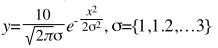
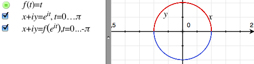
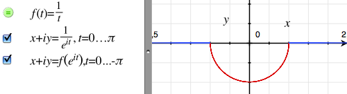
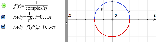
Complex numbers! Yay! If you're not familiar with them however, not to worry. We won't be needing all the complex numbers: we'll only use those that have length 1. In other words, all points on a circle of radius 1. Much simpler.

Complex numbers are 2D vectors that lead a double life. Ordinarily, they are written as the sum of two parts. Their horizontal component is a real number, a multiple of $ \class{royal}{1} $. Their vertical component, is a so-called imaginary number, a multiple of $ \class{blue}{i} $, which is a square root of -1. Which supposedly does not exist. Lies.

It is often better to see them as a length and an angle. $ \class{royal}{1} $ becomes $ \class{royal}{1∠0°} $. The number $ \class{blue}{i} $ becomes $ \class{blue}{1∠90°} $. And $ -1 $ becomes $ 1∠180° $ or $ 1∠-180° $.

When we multiply two complex numbers, their lengths multiply, and their angles add up. As the lengths are always 1 in our case, we can ignore them. Here, we multiply $ \class{orange}{1∠30°} $ by $ \class{blue}{1∠90°} $ to turn it 90° counter-clockwise. By the same rule, $ \class{blue}{1∠90°} \cdot \class{blue}{1∠90°} = 1∠180° $, better known as $ \class{blue}{i}^2 = -1 $. Complex numbers like to turn, and this gives them interesting properties, explored elsewhere on this site.

Representing 2D rotation with complex numbers is trivial. We can directly map the rotation angle to the complex number's angle, and we can combine rotations by adding up the angles, positive or negative. The angles 0°, 90°, 180°, 270°, 360° become 1, $ \class{blue}{i} $, -1, $ -\class{blue}{i} $, 1. Of course, this adds nothing useful, at least in 2D.

We can expand the model to 3D though, where we have three perpendicular ways of turning. First we'll try to add a second degree of rotation. We add a new imaginary component $ \class{green}{j} $, representing Y rotation, while $ \class{blue}{i} $ is X rotation. Any position in this 3D space is now a quaternion, but we're still limiting them to only length 1, only interested in rotation. We'll be using the surface of what is, for now, a sphere.

But wait, this isn't right. According to this diagram, if we rotate 180° around either the X or Y axis, we end up in the same place—and hence the same orientation. Clearly that's not the case. Yet we based our quaternions on complex numbers, so both $ \class{blue}{i}^2 = -1 $ and $ \class{green}{j}^2 = -1 $.

We can satisfy this condition in a different way though. If we rotate an object by 360° around any axis, we always end up back where we started. So we can make this rule work if we agree that a 360° rotation equals a 180° quaternion.

That means each rotation is represented by a quaternion of half its angle. A rotation by 180° becomes a quaternion of 90°, that is $ \class{blue}{i} $ or $ \class{green}{j} $, and each rotation axis takes us to a unique place. As we still treat $ \class{royal}{1} $ as 0°, the quaternion $ \class{blue}{1∠180°} = \class{green}{1∠180°} = -1 $ now represents a rotation of 360° = 0° around any axis. So $ \class{royal}{1} $ and $ -1 $ are considered equivalent, as far as representing rotation goes.

Furthermore, $ \class{blue}{i} $ and $ \class{slate}{-i} $ are equivalent too, and so are $ \class{green}{j} $ and $ \class{cyan}{-j} $. Each represents rotating either +180° or -180° around the corresponding axis, which is the same thing. In fact, any half of this sphere is now equivalent to the other half, when you reflect it around the central point. This is why we were missing half of the hypersphere earlier: the 'outer half' is a mirror image of the 'interior'.

So what about in-between axes? Well, we could try rotating around $ \class{orange}{(1,1,0)} $ and $ \class{gold}{(1,-1,0)} $, which are the axes that lie ±45° rotated between X and Y. We'd end up tracing circles right between them: this is the only possibility where both rotations are perpendicular, yet maintain an equal distance to both the X and Y situation.

Unfortunately we're missing something important. We've only applied rotations from neutral, from $ 1 $. If we apply a 180° X and Y rotation in series, where do we end up? And what about Y followed by X? The diagram might suggest we'd end up at respectively $ \class{green}{j} $ and $ \class{blue}{i} $.

But this wouldn't make sense: if $ \class{blue}{i} \cdot \class{green}{j} = \class{green}{j} $, and $ \class{green}{j} \cdot \class{blue}{i} = \class{blue}{i} $, then both $ \class{blue}{i} $ and $ \class{green}{j} $ have to be equal to $ 1 $. There'd be no rotation at all. And if we say that $ \class{blue}{i} \cdot \class{blue}{j} = \class{blue}{j} \cdot \class{blue}{i} = -1 $, then the quaternions $ \class{blue}{i} $ and $ \class{green}{j} $ have the exact same effect. We'd only have one imaginary dimension, not two. Even in math, a difference that makes no difference is no difference.

Whether we want to or not, we have to add a third imaginary component, $ \class{orangered}{k} $ to make this click together. So $ \class{orangered}{k}^2 = - 1 $, but it's different from both $ \class{blue}{i} $ and $ \class{green}{j} $. As we've used up our 3 dimensions, we need to project down this new 4th, putting it at an angle between the others. Again, a $ \class{orangered}{k} $ quaternion represents rotation around the Z axis, with the angle divided by two.

We end up with two peculiar relationships: $ \class{blue}{i} \cdot \class{green}{j} = \class{orangered}{k} $ and $ \class{green}{j} \cdot \class{blue}{i} = \class{purple}{-k} $. The quaternion product is not the same when you reverse the factors. Just like an XY gyroscope turns differently than a YX gyroscope. But if we'd started with Z/X or Y/Z, we'd see the exact same thing.

Hence we can rotate and combine these rules to get $ \class{blue}{i} \cdot \class{green}{j} \cdot \class{orangered}{k} = -1 $. This is the $ i^2 = -1 $ of quaternions, the magic rule that links together 3 separate imaginary dimensions and a real one, creating a maze of twisty passages all alike. When you cycle the axes, it still works: $ \class{green}{j} \cdot \class{orangered}{k} \cdot \class{blue}{i} = -1 $ and $ \class{orangered}{k} \cdot \class{blue}{i} \cdot \class{green}{j} = -1 $, demonstrating that quaternions link together three imaginary axes into a cyclic whole.

So how do we actually use quaternions for rotation? It's quite easy, because they are literally complex numbers whose imaginary component has sprouted two extra dimensions. Compare with an ordinary complex number on the unit circle. Its length (1) is divided non-linearly over the horizontal and vertical component using the cosine and sine: this is trigonometry 101.

For a quaternion on the unit hypersphere, we only make two minor changes. We replace the single $ i $ with a vector $ (x\class{blue}{i}, y\class{green}{j}, z\class{red}{k}) $ where $(x,y,z)$ is the normalized axis of rotation. The cosine and sine stay, though we divide the rotation angle by two. We can visualize the 3 imaginary dimensions directly without projection, after squishing the real dimension to nothing. As the length of the imaginary vector shrinks, the real component grows to compensate, maintaining length 1 for the entire 4D quaternion.

We can apply the rules of quaternion arithmetic to multiply two quaternions. This is equivalent to performing the rotations they represent in series. Just like complex numbers, two length 1 quaternions make another length 1 quaternion. Of course, all the other quaternions have their uses too, but they're not as common. In a graphics context, you can pretty much forget they exist.

There's only one question left: how to smoothly move between two quaternions, that is, between two arbitrary orientations. With axis-angle, it was a very complicated procedure. With quaternions, it's super easy, because unit quaternions are shaped like a hypersphere. The 'angle map' is the hypersphere itself.

As it turns out though, a hyperspherical interpolation in 4D is exactly the same as a spherical one in 3D. So we really only need to understand the 3D case. We have a linear interpolation between two points on a sphere, and want to replace it with a spherical arc.

The line and the arc share the same plane: the one that contains both points and the center of the sphere. Any such plane cuts the sphere into two equal halves, along an equator-sized great circle. Hence the arc is just an inflated version of the line, with a circular bulge applied in the plane, following the sphere's radius along the way. But we also have to traverse the arc at constant speed: otherwise we'd end up creating an uneven spline-like curve again.

Luckily, we can apply a little trigonometry again. We can use the 3D (4D) vector dot product to find the angle between two unit vectors (quaternions), after applying an arccosine. Then we weigh the two vectors (quaternions) appropriately so they sum to length 1 and move linearly with the arc length. This is the slerp, the spherical linear interpolation. Working it out yourself can be tricky, but the result is elegant and independent of the number of dimensions.

With all that in place, we can track any orientation with just 4 numbers, and change them linearly and smoothly. Quaternions are like a better axis-angle representation, which simply does the right thing all the time. Of course, you could just look up the formulas and cargo-cult your way through this problem. But it's more fun when you know what's actually going on in there. Even if it's in 4D.

So the story goes: the tortoise challenges Achilles to a footrace.

"If you give me a head start," it says, "any start at all, you can never win.".
Achilles laughs and decides to be a good sport: he'll only run twice as fast as the tortoise.

The tortoise explains: "If you want to pass me, first you have to move to where I am. By the time you get there, I'll have walked ahead a little bit."

"While you cross the next distance, I will move yet again. No matter how many times you try to catch up, I'll always be some small distance ahead. Therefor, you cannot beat me."

Achilles realizes that talking tortoises are not a sign of positive mental health, so he decides to find a wall to run into instead. It will either confirm the theory, or end the pain.

See, the race is actually unnecessary, because the problem remains the same.
In order to reach the wall, Achilles first has to cross half the way there.

Then he has to go half that distance again, and again. No matter how many times he repeats this, there will always be some distance left. So if Achilles can't cross this distance in a finite amount of steps, why is he wearing that stupid helmet?

The distance travelled forms a never ending sequence of expanding sums.
We have to examine the entire sequence, rather than individual numbers in it.

By definition, the distance travelled and distance to the wall always add up to $ 1 $. So one simple way to resolve this conundrum is to say: Well yes, it's going to take you infinitely long to glue all those pieces together, but only because you already spent an infinite amount of time chopping them up!
But that's not a very mathematically satisfying answer. Let's try something else.

The distance to the wall is always equal to the last step taken. We know that each step is half as long as the previous one, starting with $ \frac{1}{2} $. Therefor, the distance to the wall must decrease exponentially: $ \frac{1}{2}, \frac{1}{4}, \frac{1}{8}, \frac{1}{16}, … $, getting closer to zero with every step.

But why can we say that this gap effectively closes to zero after 'infinity steps'? The number that we're building up is $ \frac{1}{2} + \frac{1}{4} + \frac{1}{8} + \frac{1}{16} + … \,$

We know our sum will never exceed $ 1 $, as there is only $ 1 $ unit of distance being divided. This means $ \frac{1}{2} + \frac{1}{4} + \frac{1}{8} + \frac{1}{16} + … \leq 1 $, which eliminates every number past the surface of the wall—but not the surface itself.

Suppose we presume $ \frac{1}{2} + \frac{1}{4} + \frac{1}{8} + \frac{1}{16} + … < 1 $ and hence that this number lies some tiny distance in front of the wall.

Well in that case, all we need to do is zoom in far enough, and we'll see our sequence jump past it after a certain finite number of steps.

If we try to move it closer to the wall, the same thing happens. This number simply cannot be less than $ 1 $. Therefor $ \frac{1}{2} + \frac{1}{4} + \frac{1}{8} + \frac{1}{16} + … \geq 1 $

The only place $ \frac{1}{2} + \frac{1}{4} + \frac{1}{8} + \frac{1}{16} + … \, $ can be is exactly $ 0 $ units away from $ 1 $. If two numbers have zero distance between them, then they are equal.

What we've actually done here is applied the principle of limits: we've defined a procedure of steps that lets us narrow down the interval where the infinite sum might be. The lower bound is the sequence of sums itself: it only increases towards $ 1 $, never decreases. For the upper bound, we established no sum could exceed $ 1 $. Therefor the interval must shrink to nothing, and the sequence converges.

The purpose of a limit is then to act as a supercharged fast-forward button. It lets us avoid the infinite amount of work required to complete sums like $ \frac{1}{2} + \frac{1}{4} + \frac{1}{8} + \frac{1}{16} + … $ and simply skip to the end. To do so, we have to step back, spot the pattern, and pin down where it ends. So limits allow us to literally reach the unreachable. But in fact, you already knew that.

As soon as you learned to divide, you found $ 2 \div 3 = 0.666… = 0.6 + 0.06 + 0.006 + …\hspace{2pt} $
Even in primary school the opportunity to examine infinity is there. Rather than tackle it head on, it's simply noted and filed. Eight years later it's regurgitated in the form of cryptic epsilon-delta definitions.

But then there's those pesky consequences again. By allowing the idea of infinity, we can invent an entire zoo of paradoxical things. For example, imagine a lamp that's switched on ($1$) and off ($0$) at intervals that decrease by a factor of two: on for $ \frac{1}{2} $ second, off for $ \frac{1}{4} s $, on for $ \frac{1}{8} s $, off for $ \frac{1}{16} s $, …
After $ 1\,s $, when the switch has been flipped an infinite amount of times, is the lamp on or off?

Another way to put this is that the lamp's state at $ 1\,s $ is the result of the infinite sum $ 1 - 1 + 1 - 1 + … $
Intuitively we might say each pair of $ +1 $ and $ -1 $ should cancel out and make the entire sum equal to $ 0 $.
But we can pair them the other way, leading to $ 1 $ instead. It can't be both.

If we zoom in, it's obvious that no matter how close we get to $ 1\,s $, the lamp's state keeps switching. Therefor it's meaningless to attempt to 'fast forward' to the end, and the limit does not exist. At $ 1\,s $ the lamp is neither on nor off: it's undefined. This infinite sum does not converge.

But actually, we overcomplicated things. Thanks to the power of limits, we can ask a simpler, equivalent question. Given a lamp that switches on and off every second, what is its state at infinity? The answer's the same: it never settles.

Let's imagine the rational numbers.

Actually, hold on. Is this really a line? The integers certainly weren't connected.

Rather than assume anything, we're going to attempt to visualize all the rational numbers. We'll start with the numbers between $ 0 $ and $ 1 $.

Between any two numbers, we can find a new number in between: their average. This leads to $ \frac{1}{2} $.

By repeatedly taking averages, we keep finding new numbers, filling up the interval.

If we separate out every step, we get a binary tree.

You can think of this as a map of all the fractions of $ 2^n $. Given any such fraction, say $ \frac{13}{32} = \frac{13}{2^5} $, there is a unique path of lefts and rights that leads directly to it. At least, as long as it lies between $ 0 $ and $ 1 $.

Note that the graph resembles a fractal and that the distance to the top edge is divided in half with every step. But we only ever explore a finite amount of steps. Therefor, we are not taking a limit and we'll never actually touch the edge.

But we can take thirds as well, leading to fractions with a power of $ 3^n $ in their denominator.

As some numbers can be reached in multiple ways, we can eliminate some lines, and end up with this graph, where every number sprouts into a three-way, ternary tree. Again, we have a map that gives us a unique path to any fraction of $ 3^n $ in this range, like $ \frac{11}{27} = \frac{11}{3^3} $.

Because we can do this for any denominator, we can define a way to get to any rational number in a finite amount of steps. Take for example $ \frac{21}{60} $. We decompose its denominator into prime numbers and begin with $ 0 $ and $ 1 $ again.

There is a division of $ 2^2 $, so we do two binary splits. This time, I'm repeating the previously found numbers so you can see the regular divisions more clearly. We get quarters.

The next factor is $ 3 $ so we divide into thirds once. We now have twelfths.

For the last division we chop into fifths and get sixtieths.

$ \frac{21}{60} $ is now the 21st number from the left.

But this means we've found a clear way to visualize all the rational numbers between $ 0 $ and $ 1 $: it's all the numbers we can reach by applying a finite number of binary (2), ternary (3), quinary (5) etc. divisions, for any denominator. So there's always a finite gap between any two rational numbers, even though there are infinitely many of them.

The rational numbers are not continuous. Therefor, it is more accurate to picture them as a set of tick marks than a connected number line.

To find continuity then, we need to revisit one of our earlier trees. We'll pick the binary one.
While every fork goes two ways, we actually have a third choice at every step: we can choose to stop. That's how we get a finite path to a whole fraction of $ 2^n $.

But what if we never stop? We have to apply a limit: we try to spot a pattern and try to fast-forward it. Note that by halving each step vertically on the graph, we've actually linearized each approach into a straight line which ends. Now we can take limits visually just by intersecting lines with the top edge.

Right away we can spot two convergent limits: by always choosing either the left or the right branch, we end up at respectively $ 0 $ and $ 1 $.

These two sequences both converge to $ \frac{1}{2} $. It seems that 'at infinity steps', the graph meets up with itself in the middle.

But the graph is now a true fractal. So the same convergence can be found here. In fact, the graph meets up with itself anywhere there is a multiple of $ \frac{1}{2^n} $.

That's pretty neat: now we can eliminate the option of stopping altogether. Instead of ending at $ \frac{5}{16} $, we can simply take one additional step in either direction, followed by infinitely many opposite steps. Now we're only considering paths that are infinitely long.

But if this graph only leads to fractions of $ 2^n $, then there must be gaps between them. In the limit, the distance between any two adjacent numbers in the graph shrinks down to exactly $ 0 $, which suggests there are no gaps. This infinite version of the binary tree must lead to a lot more numbers than we might think.
Suppose we take a path of alternating left and right steps, and extend it forever. Where do we end up?

We can apply the same principle of an upper and lower bound, but now we're approaching from both sides at once. Thanks to our linearization trick, the entire sequence fits snugly inside a triangle.

If we zoom into the convergence at infinity, we actually end up at $ \class{orangered}{\frac{2}{3}} $.
Somehow we've managed to coax a fraction of $ 3 $ out of a perfectly regular binary tree.

If we alternate two lefts with one right, we can end up at $ \class{orangered}{\frac{4}{7}} $. This is remarkable: when we tried to visualize all the rational numbers by combining all kinds of divisions, we were overthinking it. We only needed to take binary divisions and repeat them infinitely with a limit.

Every single rational number can then be found by taking a finite amount of steps to get to a certain point, and then settling into a repeating pattern of lefts and/or rights all the way to infinity.

If we can find numbers between $ 0 $ and $ 1 $ this way, we can apply the exact same principle to the range $ 1 $ to $ 2 $. So we can connect two of these graphs into a single graph with its tip at $ 1 $.

But we can repeat it as much as we like. The full graph is not just infinitely divided, but infinitely big, in that no finite box can contain it. That means it leads to every single positive rational number. We can start anywhere we like. Is your mind blown yet?

No? Ok. But if this works for positives, we can build a similar graph for the negatives just by mirroring it. So we now have a map of the entire rational number set. All we need to do is take infinite paths that settle into a repeating pattern from either a positive or a negative starting point. When we do, we find every such path leads to a rational number.
So any rational number can be found by taking an infinite stroll on one of two infinite binary trees.

Wait, did I say two infinite trees? Sorry, I meant one infinitely big tree.
See, if we repeatedly scale up a fractal binary tree and apply a limit to that, we end up with almost exactly the same thing. Only this time, the two downward diagonals always eventually fold back towards $ 0 $. This creates a path of infinity + 1 steps downward. While that might not be very practical, it suggests you can ride out to the restaurant at the end of the universe, have dinner, and take a single step to get back home.

Is it math, or visual poetry? It's time to bring this fellatio of the mind to its inevitable climax.

You may wonder, if this map is so amazing, how did we ever do without?
Let's label our branches. If we go left, we call it $ 0 $. If we go right, we call it $ 1 $.

We can then identify any number by writing out the infinite path that leads there as a sequence of ones and zeroes—bits.

But you already knew that.

See we've just rediscovered the binary number system. We're so used to numbers in decimal, base 10, we didn't notice. Yet we all learned that rational numbers consist of digits that settle into a repeating sequence, a repeating pattern of turns. Disallowing finite paths works the same, even in decimal: the number $ 0.95 $ can be written as $\, 0.94999…\, $, i.e. take one final step in one direction, followed by infinitely many steps the other way.

When we write down a number digit by digit, we're really following the path to it in a graph like this, dialing the number's … er … number. The rationals aren't shaped like a binary tree, rather, they look like a binary tree when viewed through the lens of binary division. Every infinite binary, ternary, quinary, etc. tree is then a different but complete perspective of the same underlying thing. We don't have the map, we have one of infinitely many maps.

Which means we can show this graph is actually an interdimensional number portal.
See, we already know where the missing numbers are. Irrational numbers like $ π $ form a never-repeating sequence of digits. If we want to reach $ π $, we find it's at the end of an infinite path whose turns do not repeat. By allowing such paths, our map leads us straight to them. Even though it's made out of only one kind of rational number: division by two.

So now we've invented real numbers. How do we visualize this invention? And where does continuity come in? What we need is a procedure that generates such a non-repeating path when taken to the limit. Then we can figure out where the behavior at infinity comes from.

Because the path never settles into a pattern, we can't pin it down with a single neat triangle like before. We try something else. At every step, we can see that the smallest number we can still reach is found by always going left. Similarly, the largest available number is found by always going right. Wherever we go from here, it will be somewhere in this range.

We can set up shrinking intervals by placing such triangles along the path, forming a nested sequence.

What we've actually done is rounded up and down at every step, to find an upper and lower bound with a certain amount of digits. This works in any number base.

Let's examine these intervals by themselves. We can see that due to the binary nature, each interval covers either the left or right side of its ancestor. Because our graph goes on forever, there are infinitely many nested intervals. This tower of $ π $ never ends and never repeats itself, we just squeezed it into a finite space so we could see it better.

If we instead approach a rational number like $ \frac{10}{3} = 3.333…\, $ then the tower starts repeating itself at some point. Note that the intervals don't slide smoothly. Each can only be in one of two places relative to its ancestor.

In order to reach a different rational number, like $ 3.999… = 4 $, we have to establish a different repeating pattern. So we have to rearrange infinitely many levels of the tower all at once, from one configuration to another. This reinforces the notion that rational numbers are not continuous.

If the tower converges to a number, then the top must be infinitely thin, i.e. $ 0 $ units wide. That would suggest it's meaningless to say what the interval at infinity looks like, because it stops existing. Let's try it anyway.

There is only one question to answer: does the interval cover the left side, or the right?

Oddly enough, in this specific case of $ 3.999…\, $ there is an answer. The tower leans to the right. Therefor, the state of the interval is the same all the way up. If we take the limit, it converges and the final interval goes right.

But we can immediately see that we can build a second tower that leans left, which converges on the same number. We could distinguish between the two by writing it as $ 4.000…\, $ In this case the final interval goes left.

If we approach $ 10/3 $, we take a path of alternating left and right steps. The state of the interval at infinity becomes like our paradoxical lamp from before: it has to be both left and right, and therefor it is neither, it's simply undefined.

The same applies to irrational numbers like $ π $. Because the sequence of turns never repeats itself, the interval flips arbitrarily between left and right forever, therefor it is in an undefined state at the end.

But there's another way to look at this.
If the interval converges to the number $ π $, then the two sequences of respectively lower and upper bounds also converge to $ π $ individually.

Remember how we derived our bounds: we rounded down by always taking lefts and rounded up by always taking rights. The shape of the tower depends on the specific path you're taking, not just the number you reach at the end.

That means we're approaching the lower bounds so they all end in $ 0000… \, $ Their towers always lean left.

If we then take the limit of their final intervals as we approach $ π $, that goes left too. Note that this is a double limit: first we find the limit of the intervals of each tower individually, then we take the limit over all the towers as we approach $ π $.

For the same reason, we can think of all the upper bounds as ending in $ 1111 …\, $ Their towers always lean right. When we take the limit of their final intervals and approach $ π $, we find it points right.

But, we could actually just reverse the rounding for the upper and lower bounds, and end up with the exact opposite situation. Therefor it doesn't mean that we've invented a red $ π $ to the left and green $ π $ to the right which are somehow different. $ π $ is $ π $. This only says something about our procedure of building towers. It matters because the towers is how we're trying to reach a real number in the first place.

See, our tower still represents a binary number of infinitely many bits. Every interval can still only be in one of two places. To run along the real number line, we'd have to rearrange infinitely many levels of the tower all at once to create motion. That still does not seem continuous.

We can resolve this if we picture the final interval of each tower as a bit at infinity. If we flip the bit at infinity, we swap between two equivalent ways of reaching a number, so this has no effect on the resulting number.

In doing so, we're actually imagining that every real number is a rational number whose non-repeating head has grown infinitely big. Its repeating tail has been pushed out all the way past infinity. That means we can flip the repeating part of our tower between different configurations without creating any changes in the number it leads to.

That helps a little bit with the intuition: if the tower keeps working all the way up there, it must be continuous at its actual tip, wherever that really is. A continuum is then what happens when the smallest possible step you can take isn't just as small as you want. It's so small that it no longer makes any noticeable difference. While that's not a very mathematical definition, I find it very helpful in trying to imagine how this might work.

Finally, we might wonder how many of each type of number there are.
The natural numbers are countably infinite: there is a procedure of steps which, in the limit, counts all of them. Just start at the beginning, and fast-forward.

We can find a similar sequence for the even natural numbers by multiplying each number by two. We can also alternate between a positive and negative sequence to count the integers. We can match up the elements one-to-one, which means all three sequences are equally long. They're all countably infinite.
There are as many even positives as positives. Which is exactly as many as all the integers combined. As counter-intuitive as it is, it is the only consistent answer.

But we can take it one step further: we can find such a sequence for the rational numbers too, by laying out all the fractions on a grid. We can follow diagonals up and down and pass through every single one. If we eliminate duplicates like $ 1 = 2/2 = 3/3 $ and alternate positives and negatives, we can 'count them all'. So there are as many fractions as there are natural numbers. "Deal with it", says Infinity, donning its sunglasses.

The real numbers on the other hand are uncountably infinite: no process can list them all in the limit. The basic proof is short: suppose we did have a sequence of all the real numbers between $ 0 $ and $ 1 $ in some order. We could then build a new number by taking all the bits on the diagonal, and flipping zeroes and ones.
That means this number is different from every listed number in at least one digit, so it's not on the list. But it's also between $ 0 $ and $ 1 $, so it should be on the list. Therefor, the list can't exist.

This even matches our intuitive explanation from earlier. There are so many real numbers, that we had to invent a bit at infinity to try and count them, and find something that would tick at least once for every real number. Even then we couldn't say whether it was $ 0 $ or $ 1 $ anywhere in particular, because it literally depends on how you approach it.

We're going to go for a drive.

We'll graph speed versus time. We have kilometers per hour vertically, and hours horizontally. We've also got a speedometer—how fast—and an odometer—how far.

Suppose we drive for half an hour at 50 km/h.

We end up driving for 25 km. This is the area of spanned by the two lengths: $ 50 \cdot \frac{1}{2} $, a rectangle.

Now we hit the highway and maintain 120 km/h for the rest of the hour. We go an additional 60 km, the area of the second rectangle, $ 120 \cdot \frac{1}{2} $.
Whenever we multiply two units like speed and time, we can always visualize the result as an area.

Because we crossed 85 km in one hour, this is equivalent to driving at a constant speed of 85 km/h for the duration. The total area is the same.

If this were a race between two different cars, we would see a photo finish. The distance travelled in kilometers is identical at the 1 hour mark. Where they differ is in their speed along the way, with the red car falling behind and then catching up.

The difference is visible in the slope of both paths. The faster the car, the more quickly it accumulates kilometers. If it drove 25 km in half an hour, then its speed was 50 km/h, $ \frac{25}{0.5} $. This is the distance travelled divided by the time it took, vertical divided by horizontal.

Slope is a relative thing. If we shrink the considered time, the distance shrinks along with it, and the resulting speed is the same. What we're really doing is formalizing the concept of a rate of change, of distance over time.

Constant speed means a constant increase in distance. We can directly relate the area being swept out left to right with the accumulated distance by each car. This is clue number 1.

Now suppose the red car starts ahead by 10 km and drives the same speeds.
It will also end up 10 km ahead after 1 hour, its path has simply been shifted by 10 units. The slope is unchanged: it doesn't matter where you are and where you've been, only how fast you're going right now. It's what's called an instantaneous quantity, it describes a situation only in the moment. This is clue number 2.

In order to get ahead, the red car had to drive there. So we can imagine it started earlier, $ \frac{1}{5} $ of an hour, driving for 10 km at the same speed. Again, the equality holds: area swept out equals accumulated distance, we add another $ 50 \cdot \frac{1}{5} $. Constant slope still equals constant speed.

One curve describes how the other changes in the moment, therefor the two quantities are linked somehow. We add up area to go from speed to distance; we find slope to go from distance to speed. We're going to examine this two-way relationship more.

Real cars don't start or stop on a dime, they accelerate and decelerate. So we're going to try more realistic behavior.

Suppose the speed follows a curve. In one hour, the car starts from 0 km/h, accelerates to over 100 km/h and then smoothly decelerates back to standstill. The distance travelled also curves smoothly, from 0 to 60 km, so we've driven 60 km in total.

We can immediately see that at the point where the car was going fastest, the distance was increasing the most. Its slope is steepest at that point. The relationship between the two curves holds.

But actually measuring it is a problem. First, there are no more straight sections to measure the slope on. If we take two points on a curve, the line that connects them doesn't touch the curve, it crosses it at an angle.

Second, we can no longer measure the area by dividing it into rectangles, or any other simple geometric shape. There will always be gaps. We can solve both of these problems with a dash of infinity.

We'll start with area. We have to find an upper and a lower bound again.
We're going to divide the curve into 4 sections.

First, the upper bound. We find the highest value in each section and make a rectangle of that height. This approach is too greedy and overestimates.

The lower bound is similar. We find the smallest value in each interval and make rectangles of that height.
This underestimates and leaves areas uncovered.

If we do 7 divisions instead. We can see that the upper bound has decreased: there is less excess area. The lower bound has increased: the gaps are smaller and more area is covered.

With 10 divisions, it's even better. It seems the upper and lower bounds are approaching each other.

And the same at 13 divisions. If we keep doing this, our slices will get thinner and thinner, and we'll be adding more of them together. If we take a limit, each slice becomes infinitely thin, and there are infinitely many of them. Let's step back and see what that means.

Take for example the sequence of lower bounds.

Because every slice is equally wide, we can glue them together into a single rectangle per step.
Its width $ w $ is the thickness of a single slice, and its height $ h $ is the sum of the heights of the slices.

In the limit, this rectangle becomes both infinitely thin and infinitely tall. This is a tug of war between Zero and Infinity where at first sight, they both seem to win. That's a problem. Luckily, we're not interested in the rectangle itself, but rather its area.

We can change a rectangle's sides without changing its area. We multiply its width by one factor (e.g. $ 2 $), and divide the height by the same amount. The area $ 2w \cdot \frac{h}{2} $ is unchanged. Hence, we can normalize our rectangles to all have the same width, for example $ 1 $.

We can do the same for the upper bounds. We can see that both areas are converging on the same value. This is the true area under the curve, which is neither zero nor infinite. In this tug of war, both parties are equally matched.

Now our sequence looks very different: it's approaching a definite area, sandwiched between red and blue.

If we take the limit, we get the area under our curve.

This way we can find the area under any smooth curve. This process is called integration. The symbol for integration is $ \int_a^b $ where $ a $ and $ b $ are the start and end points you're integrating between. The S-shape stands for our sum, adding up infinitely many pieces.

We can then integrate one curve to make another, by sweeping out area horizontally from a fixed starting point. We move the end point to a time $ T $ and plot the accumulated value along the way. Using limits, we can do this continuously. This takes us from speed to distance travelled. The quantity $ \,\mathrm{d}t\, $ is the infinitesimal width of each slice, an infinitely small amount of time.

Now we just need to figure out the reverse and find slopes. We'll go back to our failed attempt from earlier.

If we shrink the distance we're considering, our slope estimate gets closer to the true value. But if we try to take a limit, we end up dividing $ 0 $ by $ 0 $.

Instead we need to normalize our sequence again so it doesn't vanish.

We only care about slope: the ratio of the two right sides. Which means, if we scale up each triangle, the ratio is unchanged. That just comes down to multiplying both sides by the same number. Again we can scale them all to the exact same width.

Now we've created a limit that does converge to something rather than nothing.

This finite value is the slope at the point we were homing in on. Because we can apply this process at any point on the curve, we can find the exact slope anywhere. This is called finding the derivative or differentiation.

We can also apply this process over an entire curve to generate a new one. So now we know how to go the other way: distance to speed. Mathematically, we are dividing an infinitesimal piece of the distance, $ \,\mathrm{d} \class{slate}{f(t)}\, $, by an infinitesimal slice of time $ \,\mathrm{d} t\, $. Working with infinitesimal formulas is tricky however. There's always an implied limit being taken in order to reach them in the first place. Indeed, it took centuries to formalize this fuzzy explanation into what we call differential forms today.

We can note that if we shift the distance curve up or down, the speed is unchanged. When you take a derivative, any constant value you've added to your function simply disappears. This shows again that speed is always in the moment, it only describes what's going on in an infinitely short piece of curve.

Differentiation is then like x-ray specs for curves and quantities, and it's turtles all the way down. For example, if we differentiate speed, we get acceleration. This is another rate of change, of speed over time. We see the car's acceleration is initially positive, speeding up, and then goes negative, to slow down, i.e. accelerate in the opposite direction.
Note: The acceleration has been divided by 4 to fit.

If we integrate acceleration to get speed, we have to count the second part as negative area: it is causing the speed to decrease.

We can see that the point of maximum speed is the point where the acceleration passes through $ 0 $. One of the most useful applications of derivatives is indeed to find a maximum or minimum of a curve more easily. No matter where it is, the slope at such a point must always be horizontal—provided the curve is smooth.

Let's end this with a more exciting example. What's tall, fast and makes kids scream?

A roller coaster! We'll construct a little track by welding together pieces of circles and lines.

Alas, we shouldn't be too proud of our creation. Even though it looks smooth, there's something very wrong. This is how you build roller coasters when you don't want people to have fun. To see the problem, we need to use our x-ray specs.

We differentiate the height into its slope. It has sharp corners all over the place. Even though the track itself looks smooth, it doesn't change smoothly. The slope is constant in the straight sections and changes rapidly in the curved sections.

If we take the derivative of the slope, i.e. find the slope's slope, we get a measure of curvature. It's positive inside valleys, negative on top of crests. This graph is even worse: there are sharp peaks and cliffs. Note that in the formula, we are now dividing by the square of the infinitesimal distance $ \mathrm{d}x $. This is like going two levels down on the hyperreal number line and back up again.

We can see better if we replace the second derivative with the 2D curvature.
This is the radius of the circle that touches the curve at a given point. As this radius gets infinitely big on straight sections, we use its inverse, $ \class{teal}{κ} $. Because of how we built the track, $ κ $ switches between $ 0 $ and a constant positive or negative value.
At every switch, there will be a corresponding change in force, a jerk.

Let's simulate a ride. As riders go through our curved sections, their inertia will push them to the outside of the curve. From their point of view, this is a centrifugal force up or down. We'll plot the (subjective) vertical G force including gravity. It starts at a comfy 1 G, but then swings wildly between 0.5 G and 1.25 G.

Even though the track seems smooth, we can see that the vertical G's are not. Every time we enter a curve, we experience a sudden jerk up or down. This is due to the jumps in the curvature. The G's are themselves curved, because the rider's sense of gravity decreases as the cart goes vertical. The sharp dips below 0.5 G are not simulation errors: this is actually what it would feel like.

To really highlight the problem, we need to x-ray the G's and derive again. G forces are a form of acceleration. The derivative of acceleration is a change in force, called jerk. Whenever it's non-zero, you feel jerked in a particular direction.

To fix this, we need to alter the curve of the track and smooth it out at all the different levels of differentiation. Here I've applied a relaxation procedure. It's like a blur filter in photoshop: we replace every point on the track with the average of its neighbours. We get a subtly different curve. Its height hasn't changed much at all, it's just a little bit less tense.

But this minor change has a huge effect on both slope and radius of curvature. They are completely smoothed out, with all corners and jumps removed.

If we do another simulation, the G force graph looks completely different. There are no more jumps.

But the real difference is in jerk. There are no more actual jerks, only smooth oscillations. Instead of bruises, riders will get butterflies. Thanks to calculus, we avoided that painful lesson without ever having to ride it ourselves.

Please check your pockets for loose items. Lost property will not be returned.

Let's start with the original, unrelaxed track. Thanks to calculus, we can simulate head-bobbing so you can get a feel for how jerky this is. Even virtually, this isn't very pleasant.

This is the improved track. Notice the smooth transitions in and out of curves.

And that's how you make sweet roller coasters: by building them out of infinitely small, smooth pieces, so you don't get jerked around too much.

We'll start with the classic real number line, marked at the integer positions, and poke around.
We imagine the line continues to the left and right indefinitely.

But there's a problem with this visualization: by picturing numbers as points,
it's not clear how they act upon each other.
For example, the two adjacent numbers $ \class{blue}{2} + \class{green}{3} $ sum to $ \class{red}{5} $ …

… but the similarly adjacent pair $ \class{blue}{-2} + \class{green}{-1} = \class{red}{-3} $.
We can't easily spot where the red point is going to be based on the blue and green.

A better solution is to represent our numbers using arrows instead, or vectors.
Each arrow represents a number through its length, pointing right/left for positive/negative.

The nice thing about arrows is that you can move them around without changing them.
To add two arrows, just lay them end to end. You can easily spot why $ \class{blue}{-2} + \class{green}{-1} = \class{red}{-3} $ …

… and why $ \class{blue}{2} + \class{green}{3} = \class{red}{5} $, similarly.
As long as we apply positives and negatives correctly, everything still works.

Now let's examine multiplication. We're going to start with $ \class{blue}{1} $ and then we'll multiply it by $ \class{green}{1.5} $ repeatedly.

With every multiplication, the vector gets longer by 50 percent.
These vectors represent the numbers $ \class{red}{1}, \class{red}{1.5}, \class{red}{2.25}, \class{red}{3.375} $, $ \class{red}{5.0625} $, a nice exponential sequence.

Now we're going to do the same, but multiplying by the negative, $ \class{green}{-1.5} $, repeatedly.

The vectors still grow by 50%, but they also flip around, alternating between positive and negative.
These vectors represent the sequence $ \class{red}{1}, \class{red}{-1.5}, \class{red}{2.25}, \class{red}{-3.375}, \class{red}{5.0625} $.

But there's another way of looking at this. What if instead of flipping from positive to negative, passing through zero, we went around instead, by rotating the vector as we're growing it?

We'd get the same numbers, but we've discovered something remarkable: a way to enter and pass through the netherworld around the number line. The question is, is this mathematically sound, or plain non-sense?

The challenge is to come up with a consistent rule for applying these rotations. We start with normal arithmetic. Multiplying by a positive didn't flip the sign, so we say we rotated by $ 0^\circ $. Multiplying by a negative flips the sign, so we rotated by $ \class{green}{180^\circ} $. The lengths are multiplied normally in both cases.

Now suppose we pick one of the in-between nether-numbers, say the vector of length $ 1.5 $, at a $ 90^\circ $ angle. What does that mean? That's what we're trying to find out! We'll write that as $ \class{green}{1.5 \angle 90^\circ} $ (1.5 at 90 degrees). It could make sense to say that multiplying by this number should rotate by $ \class{green}{90^\circ} $ while again growing the length by 50%.

This creates the spiral of points: $ \class{red}{1 \angle 0^\circ} $, $ \class{red}{1.5 \angle 90^\circ} $, $ \class{red}{2.25 \angle 180^\circ} $, $ \class{red}{3.375 \angle 270^\circ} $, $ \class{red}{5.0625 \angle 360^\circ} $. Three of those are normal numbers: $ +1 $, $ -2.25 $ and $ +5.0625 $, lying neatly on the real number line. The other two are new numbers conjured up from the void.

Let's examine this rotation more. We can pick $ 1 $ at a $ \class{green}{45^\circ} $ angle. Multiplying by a $ 1 $ probably shouldn't change a vector's length, which means we'd get a pure rotation effect.

By multiplying by $ \class{green}{1 \angle 45^\circ} $, we can rotate in increments of $ 45^\circ $.
It takes 4 multiplications to go from $ +1 $, around the circle of ones, and back to the real number $ -1 $.

And that's actually a remarkable thing, because it means our invented rule has created a square root of $ -1 $.
It's the number $ \class{green}{1 \angle 90^\circ} $.

If we multiply it by itself, we end up at angle $ \class{green}{90} + \class{green}{90} = \class{blue}{180^\circ} $, which is $ \class{blue}{-1} $ on the real line.

But actually, the same goes for $ \class{green}{1 \angle 270^\circ} $.

When we multiply it by itself, we end up at angle $ \class{green}{270} + \class{green}{270} = \class{blue}{540^\circ} $. But because we went around the circle once, that's the same as rotating by $ \class{blue}{180^\circ} $. So that's also equal to $ \class{blue}{-1} $.

Or we could think of $ +270^\circ $ as $ -90^\circ $, and rotate the other way. It works out just the same. This is quite remarkable: our rule is consistent no matter how many times we've looped around the circle.

Either way, $ \class{blue}{-1} $ has two square roots, separated by $ 180^\circ $, namely $ \class{green}{1 \angle 90^\circ} $ and $ \class{green}{1 \angle 270^\circ} $.
This is analogous to how both $ 2 $ and $ -2 $ are square roots of $ 4 $.

Complex multiplication can then be summarized as: angles add up, lengths multiply, taking care to preserve clockwise and counterwise angles. Above, we multiply two random complex numbers a and b to get c.

When we start changing the vectors, c turns along, being tugged by both a and b's angles. It wraps around the circle, while its length changes. Hence, complex numbers like to turn, and it's this rule that separates them from ordinary vectors.

We can then picture the complex plane as a grid of concentric circles. There's a circle of ones, a circle of twos, a circle of one-and-a-halfs, etc. Each number comes in many different versions or flavors, one positive, one negative, and infinitely many others in between, at arbitrary angles on both sides of the circle.

Which brings us to our reluctant and elusive friend, $ \class{blue}{i} $. This is the proper name for $ \class{blue}{1 \angle 90^\circ} $, and the way complex numbers are normally introduced: $ i^2 = -1 $. The magic is that we can put a complex number anywhere a real number goes, and the math still works out, oddly enough. We get complex answers about complex inputs.

Complex numbers are then usually written as the sum of their (real) X coordinate, and their (imaginary) Y coordinate, much like ordinary 2D vectors. But this is misleading: the ugly number $ \class{red}{\frac{\sqrt{3}}{2} + \frac{1}{2}i } $ is actually just $ \class{green}{1 \angle 30^\circ} $ in disguise, and it acts more like a $ 1 $ than a $ \frac{1}{2} $ or $ \frac{\sqrt{3}}{2} $. While knowing how to convert between the two is required for any real calculations, you can cheat by doing it visually.

But looking at individual vectors only gets us so far. We study functions of real numbers by looking at a graph that shows us every output for every input. To do the same for complex numbers, we need to understand how these numbers-that-like-to-turn, this field of vectors, change as a whole.
Note: from now on, I'll put $ +1 $, i.e. $ 0^\circ $ at the 12 o'clock position for simplicity.

When we apply a square root, each vector shifts. But really, it's the entire fabric of the complex plane that's warping. Each circle has been squeezed into a half-circle, because all the angles have been halved—the opposite of squaring, i.e. doubling the angle. The lengths have had a normal square root applied to them, compressing the grid at the edges and bulging it in the middle.

But remember how every number had two opposite square roots? This comes from the circular nature of complex math. If we take a vector and rotate it $ 360 ^\circ $, we end up in the same place, and the two vectors are equal. But after dividing the angles in half, those two vectors are now separated by only $ 180 ^\circ $ and lie on opposite ends of the circle. In complex math, they can both emerge.

Complex operations are then like folding or unfolding a piece of paper, only it's weird and stretchy and circular. This can be hard to grasp, but is easier to see in motion. To help see what's going on, I've cut the disc and separated the positive from the negative angles in 3D.

When we square our numbers to undo the square root, the angles double, folding the plane in on itself. The lengths are also squared, restoring the grid spacing to normal.

After squaring, each square root has now ended up on top of its identical twin, and we can merge everything back down to a flat plane. Everything matches up perfectly.

Thus the square root actually looks like this. New numbers flow in from the 'far side' as we try and shear the disc apart. The complex plane is stubborn and wants to stay connected, and will fold and unfold to ensure this is always the case. This is one of its most remarkable properties.

There's no limit to this folding or unfolding. If we take every number to the fourth power, angles are multiplied by four, while lengths are taken to the fourth power. This results in 4 copies of the plane being folded into one.

However, things are not always so neat. What happens if we were to take everything to an irrational power, say $ \frac{1}{\sqrt{2}} $? Angles get multiplied by $ 0.707106... $, which means a rotation of $ 360^\circ $ now becomes $ \sim 254.56^\circ $.

Because no multiple of $ 360 $ is divisible by $ \frac{1}{\sqrt{2}} $, the circular grid never matches up with itself again no matter how far we extend it. Hence, this operation splits a single unique complex number into an infinite amount of distinct copies.

For any irrational power $ p $, there are an infinite number of solutions to $ z^p = c $, all lying on a circle. For a hint as to why this is so, we can look at Taylor series: an arbitrary function $ f(z) $ can be written as an infinite sum $ a + bz + cz^2 + dz^3 + ... \,$ When z is complex, such a sum doesn't just represent a finite amount of folds, but a mindboggling infinite origami of complex space.

Our region of interest is the disc of complex numbers less than $ 2 $ in length. I've marked the circle of ones as a reference.

We take an arbitrary set of numbers, like this grid, and start applying the formula $ f(z) = z^2 + c $ to each. Rather than use vectors, I'll just draw points, to avoid cluttering the diagram.

First we square each number. That is, their lengths are squared, their angles are doubled.
The squaring has a dual effect: numbers larger than $ 1 $ grow bigger and are pushed outwards, numbers less than $ 1 $ grow smaller and are pulled inwards.

Next, we reset the grid back to neutral, keeping the numbers in their new place.
We also pick a random value for the constant $ \class{green}{c} $, e.g. $ \class{green}{0.57 \angle -59^\circ} $.

Now we add $ \class{green}{c} $ to each point, completing one round of Julia iteration, $ f(z) = z^2 + c $. As a result, some numbers have ended up closer towards the origin (i.e. $ 0 $), others further away from it. The combination of folding + shifting has had a non-obvious effect on the numbers.

We begin the second iteration and square each number again. Any number not inside the critical circle of $ 1 $ in the middle will get pushed out again. The other numbers continue to linger in the middle.

If we zoom out, we can see the larger numbers are spiralling outwards and are permanently lost. The minor nudge by $ \class{green}{c} $ won't be enough to bring them back.

Others remain in the middle, being drawn in, but are also at risk of being pushed out of the circle by $ \class{green}{c} $.

Resetting the grid again, we add the same value $ \class{green}{c} $ to our vectors again to finish. At this point, our original grid of numbers has been completely jumbled up.

If we continued this process would any numbers remain in the middle? Or would they eventually all get flung out? Unfortunately it's very hard to see what's going on while iterating forwards, because we lose track of where each point came from.

So we're going to go backwards instead. We'll establish a safe-zone of all numbers less than $ 2 $, forming a solid disc of all those which aren't irretrievably lost. We want to know where all these numbers can possibly come from. To help track these points, I've coloured one area in a different shade.

First we have to shift the numbers again, this time in the opposite direction to subtract $ c $.

Now we apply the square root to find $ z_{n-1} = \pm \sqrt{z_n - c} $, which is a Julia iteration in reverse.

After one backwards iteration, the disc has been squished down into an oval at an angle.
These are all the points that will definitely stay in the middle after one iteration.

When we apply the second iteration, a pattern starts to develop. Because of the repeated unfolding, we create two bulges wherever there was previously only one.

At the same time, the square root alters the length of each number as well. As a result, we squeeze in the radial direction, scaling down earlier features as they combine with newly created ones.

After 4 iterations, we start to see the first hints of self-similarity. The shape's lobes are sprouting into spirals.

But all we've really done is narrow down our blue safe-zone to include only those points that 'survive' up to 5 Julia iterations.

Remarkably this seems to distort the fractal evenly: our highlighted circles don't stretch into ovals. This is not a coincidence. Complex operations are indeed stubborn, in that they all preserve right angles everywhere. To do so, the mapping must act like a pure scaling and rotation at every point, without shearing off in any particular direction. This is what allows the fractal to look like itself at different scales.

Skipping ahead to iteration 12, we've definitely abandoned the realm of neat, traditional geometry.
Despite curving wildly, the total mapping $ z_{12} $ still has this property of evenness, which is properly referred to as a conformal mapping.

After 128 iterations, we end up with this intricate dragon-like shape, approximating the safe zone for the true fractal map $ z_\infty $. The numbers that make up the blue area are the hardiest points that will survive the next 128 attempts on their life. All the others will definitely get flung out.

Yet this complicated shape is merely the result of folding over and over again, adding a simple constant in between. If we perform a forwards Julia iteration, i.e. squaring and shifting, we see this shape matches up with itself, and looks identical before and after.

For different values of $ \class{green}{c} $, the fractal morphs into other shapes. There's literally an infinite variety to discover. Some sets are made up of disconnected parts. In this case, $ |c| $ is large enough to push the solid disc away from the center in a single iteration, but not so far that some points can't fold back in. If $ |c| $ gets much larger, the set vanishes.

For a smaller $ c $, Julia sets are solid. Even a small shift in the value of $ c $ can accumulate into a large difference. Here we zone in on some fluffy clouds right outside the 'solid zone'. Oddly enough, it seems when $ c $ is not inside of its own Julia set, the set is not solid. Note that in this case, 128 iterations is not sufficient: large solid patches remain, which would be divided further with more iterations.

This area of fractal space is dubbed Seahorse Valley, for rather obvious reasons.

Nearby, we find these jewel-like spirals.

Buried deep inside, there are remarkable combinations of shapes, like this pearl necklace covered in something resembling palm trees.

And we can even make snowflakes. The dramatic changes due to $ c $ reveal the chaotic nature of fractals. Mathematically, chaos occurs when even the tiniest change can accumulate and blow up to an arbitrarily large effect.

If we change our iteration formula, for example to a fourth power $ f(z) = z^4 + c $, the entire shape changes. Because each iteration now turns one bulge into four, the resulting shape has four-fold rotational symmetry.

Again, different values of $ \class{green}{c} $ make different shapes, precipitating dramatic changes.

To understand the effect of $ c $ we need to make a Mandelbrot set. This is similar to a Julia set, but the formula is applied differently. We'll use $ z^2 + c $ again. Instead of different starting values $ z_1 $, we choose different values of $ c $ and start with $ z_1 = 0 $ every time. Because $ c $ is no longer constant, the mapping stops being a simple folding operation. Each iteration is now unique and not so easy to visualize.

Because the Mandelbrot set traverses all possible values of $ c $ across its surface, it has a part of every associated Julia set in it. Around any number $ \class{green}{c} $ it looks like the Julia set which has that value as its constant. Here, we move towards the three-way cross at the bottom of the Mandelbrot set. The Julia set develops similar features.

Where the Mandelbrot set is round and bulbous, the Julia set is too.

The spirals and seahorses from earlier are located here. You can literally see the shapes on both sides of the valley evolving towards horseheads and spirals respectively. But the Mandelbrot set acts like a map to Julia sets in a much more direct way: anywhere the Mandelbrot set is filled in (blue), the corresponding Julia set is solid too. The white areas are values of $ c $ which create disconnected Julia sets.

That the Mandelbrot set is a 'pixel-perfect' map of Julia sets is a big clue. It reflects that they're actually both slices of a single higher dimensional object. By viewing these slices as we travel through, we can get a vague idea of its shape and complexity. In this object, every point in the Mandelbrot set is connected to the center of the corresponding Julia set. Actually picturing this 4D object is a challenge.

But like any fractal, the Mandelbrot set also contains copies of itself, buried inside its edge. This is just one of the many varied copies. As a result, deep Mandelbrot zooms can reach astonishing levels of beauty in complexity. This is best done with specialized software that can calculate with hundreds of digits of precision.

Take for example a sine wave $ w(x) $.

For the wave to propagate across a distance, its values have to ripple up and down over time.
The rate of change over time is drawn on top. This is the vertical velocity at every point. Both the wave and its rates of change undergo a complicated numerical dance.

But to properly describe this motion, we have to go one level deeper. We have to examine the rate of change of the vertical velocity of the wave. This is its vertical acceleration. We see that green vectors tug on blue vectors as blue vectors tug on the wave.

It's easier to see what's going on if we center the vectors vertically. The acceleration appears to be equal but opposite to the wave itself.

But that's just a lucky coincidence. If we shift the wave up by one unit, its opposite shifts down by a unit. Yet its velocity and acceleration are unaltered. So acceleration is not simply the opposite of the wave.

What's actually going on is that the green vectors match the curvature of the wave, positive inside valleys, negative on top of crests. Intuitively, this can be explained by saying that waves tend to bounce towards an average level: this is going to pull the value up out of valleys and down from peaks.

But curvature is the rate of change of the slope, and slope is the rate of change over a distance. So to describe real waves, we need to relate 'second level' change over time and change over distance, each deriving twice. This is Complicated with a capital C.

Let's try this with complex numbers instead. Until now, we had a 2D graph, showing the real value of the wave over real distance. We're going to make the wave's value complex. Mapping a 1D number (distance) to a 2D number (the wave function), means we need a 3D diagram.

The complex plane is mapped into the old Y direction (real) and the new Z direction (imaginary).

To make a complex wave, we do the thing complex numbers are best at: we make them turn, and make a helix. In this case, our wave function is simply the variable number $ 1 \angle x $ , a constant length with a smoothly changing rotation over distance.

To make the wave move, we can simply twist it in-place. Which we now know is the same as multiplying by an increasing angle $ 1 \angle t $. If we plot the complex velocity of each point, at first sight this might not look any simpler than the real wave. But in fact, these vectors are not changing in length at all, unlike the real version. As the wave is pulled by the velocity vectors, both undergo a pure rotation.

At all times, the velocity is offset by $ 90^\circ $ from the wave itself. And that means that described in complex numbers, wave equations are super easy. Instead of involving two derivatives, i.e. the rate of rate of change, we only need one. There is a direct relationship between a value and its rate of change. The necessary rotation by $ 90^\circ $ can then be written simply as multiplying by $ i $.

To recover a real wave from a complex wave, we can simply flatten it back to 2D, discarding the imaginary part. By using complex numbers to describe waves, we give them the power to rotate in place without changing their amplitude, which turns out to be much simpler.

In fact, flattening the wave has a perfectly reasonable complex interpretation: it's what happens when we average out a counter-clockwise wave (positive frequency) with a clockwise wave (negative frequency). By twisting each in opposite directions, the combined wave travels along, locked to the real number line.

But if we add up two arbitrary complex frequencies, their sum immediately turns into a spirograph pattern that manages to evolve and propagate, even as it just rotates in place. Though the original waves both had a constant amplitude of $ 1 $, the relative differences in angles (i.e. the phase) allows them to cancel out in surprising ways.

Neither curve is actually moving forward: they're just spinning in place, creating motion anyway. This is actually what quantum superposition looks like, where two or more complex probability waves combine and interfere. Where the result cancels out to zero, that's where two separate possible states are cancelling out each other, creating interference. That the underlying numbers are complex doesn't prevent them from describing real physics, indeed, it seems that's how nature actually works.

This serene display hides a whirlwind of phase. We can plot the velocity of the two frequencies, and their combination, scaled down for clarity. Once again you can see the power of describing waves with complex numbers, letting you split up a complicated motion into simple, repetitive rotations… into numbers that like to turn.