Frequency-domain blue noise generator
In computer graphics, stochastic methods are so hot right now. All rendering turns into calculus, except you solve the integrals by numerically sampling them.
As I showed with Teardown, this is all based on random noise, hidden with a ton of spatial and temporal smoothing. For this, you need a good source of high quality noise. There have been a few interesting developments in this area, such as Alan Wolfe et al.'s Spatio-Temporal Blue Noise.
This post is about how I designed noise in frequency space. I will cover:
- What is blue noise?
- Designing indigo noise
- How swap works in the frequency domain
- Heuristics and analysis to speed up search
- Implementing it in WebGPU
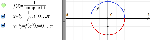
Along the way I will also show you some "street" DSP math. This illustrates how getting comfy in this requires you to develop deep intuition about complex numbers. But complex doesn't mean complicated. It can all be done on a paper napkin.

The WebGPU interface I built
What I'm going to make is this:
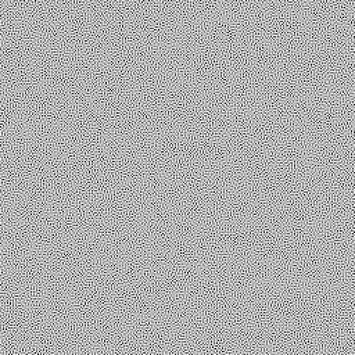
If properly displayed, this image should look eerily even. But if your browser is rescaling it incorrectly, it may not be exactly right.
Colorless Blue Ideas
I will start by just recapping the essentials. If you're familiar, skip to the next section.
Ordinary random generators produce uniform white noise: every value is equally likely, and the average frequency spectrum is flat.

Time domain

Frequency domain
To a person, this doesn't actually seem fully 'random', because it has clusters and voids. Similarly, a uniformly random list of coin flips will still have long runs of heads or tails in it occasionally.
What a person would consider evenly random is usually blue noise: it prefers to alternate between heads and tails, and avoids long runs entirely. It is 'more random than random', biased towards the upper frequencies, i.e. the blue part of the spectrum.

Time domain

Frequency domain
Blue noise is great for e.g. dithering, because when viewed from afar, or blurred, it tends to disappear. With white noise, clumps remain after blurring:

Blurred white noise

Blurred blue noise
Blueness is a delicate property. If you have e.g. 3D blue noise in a volume XYZ, then a single 2D XY slice is not blue at all:

XYZ spectrum

XY slice

XY spectrum
The samples are only evenly distributed in 3D, i.e. when you consider each slice in front and behind it too.
Blue noise being delicate means that nobody really knows of a way to generate it statelessly, i.e. as a pure function f(x,y,z). Algorithms to generate it must factor in the whole, as noise is only blue if every single sample is evenly spaced. You can make blue noise images that tile, and sample those, but the resulting repetition may be noticeable.
Because blue noise is constructed, you can make special variants.
Uniform Blue Noise has a uniform distribution of values, with each value equally likely. An 8-bit 256x256 UBN image will have each unique byte appear exactly 256 times.
Projective Blue Noise can be projected down, so that a 3D volume XYZ flattened into either XY, YZ or ZX is still blue in 2D, and same for X, Y and Z in 1D.
Spatio-Temporal Blue Noise (STBN) is 3D blue noise created specifically for use in real-time rendering:
- Every 2D slice XY is 2D blue noise
- Every Z row is 1D blue noise
This means XZ or YZ slices of STBN are not blue. Instead, it's designed so that when you average out all the XY slices over Z, the result is uniform gray, again without clusters or voids. This requires the noise in all the slices to perfectly complement each other, a bit like overlapping slices of translucent swiss cheese.
This is the sort of noise I want to generate.

Indigo STBN 64x64x16

XYZ spectrum
Sleep Furiously
A blur filter's spectrum is the opposite of blue noise: it's concentrated in the lowest frequencies, with a bump in the middle.

If you blur the noise, you multiply the two spectra. Very little is left: only the ring-shaped overlap, creating a band-pass area.

This is why blue noise looks good when smoothed, and is used in rendering, with both spatial (2D) and temporal smoothing (1D) applied.
Blur filters can be designed. If a blur filter is perfectly low-pass, i.e. ~zero amplitude for all frequencies > $ f_{\rm{lowpass}} $ , then nothing is left of the upper frequencies past a point.
If the noise is shaped to minimize any overlap, then the result is actually noise free. The dark part of the noise spectrum should be large and pitch black. The spectrum shouldn't just be blue, it should be indigo.
When people say you can't design noise in frequency space, what they mean is that you can't merely apply an inverse FFT to a given target spectrum. The resulting noise is gaussian, not uniform. The missing ingredient is the phase: all the frequencies need to be precisely aligned to have the right value distribution.
This is why you need a specialized algorithm.
The STBN paper describes two: void-and-cluster, and swap. Both of these are driven by an energy function. It works in the spatial/time domain, based on the distances between pairs of samples. It uses a "fall-off parameter" sigma to control the effective radius of each sample, with a gaussian kernel.
$$ E(M) = \sum E(p,q) = \sum \exp \left( - \frac{||\mathbf{p} - \mathbf{q}||^2}{\sigma^2_i}-\frac{||\mathbf{V_p} - \mathbf{V_q}||^{d/2}}{\sigma^2_s} \right) $$

STBN (Wolfe et al.)
The swap algorithm is trivially simple. It starts from white noise and shapes it:
- Start with e.g. 256x256 pixels initialized with the bytes 0-255 repeated 256 times in order
- Permute all the pixels into ~white noise using a random order
- Now iterate: randomly try swapping two pixels, check if the result is "more blue"
This is guaranteed to preserve the uniform input distribution perfectly.
The resulting noise patterns are blue, but they still have some noise in all the lower frequencies. The only blur filter that could get rid of it all, is one that blurs away all the signal too. My 'simple' fix is just to score swaps in the frequency domain instead.
If this seems too good to be true, you should know that a permutation search space is catastrophically huge. If any pixel can be swapped with any other pixel, the number of possible swaps at any given step is O(N²). In a 256x256 image, it's ~2 billion.
The goal is to find a sequence of thousands, millions of random swaps, to turn the white noise into blue noise. This is basically stochastic bootstrapping. It's the bulk of good old fashioned AI, using simple heuristics, queues and other tools to dig around large search spaces. If there are local minima in the way, you usually need more noise and simulated annealing to tunnel over those. Usually.
This set up is somewhat simplified by the fact that swaps are symmetric (i.e. (A,B) = (B,A)), but also that applying swaps S1 and S2 is the same as applying swaps S2 and S1 as long as they don't overlap.
Good Energy
Let's take it one hurdle at a time.
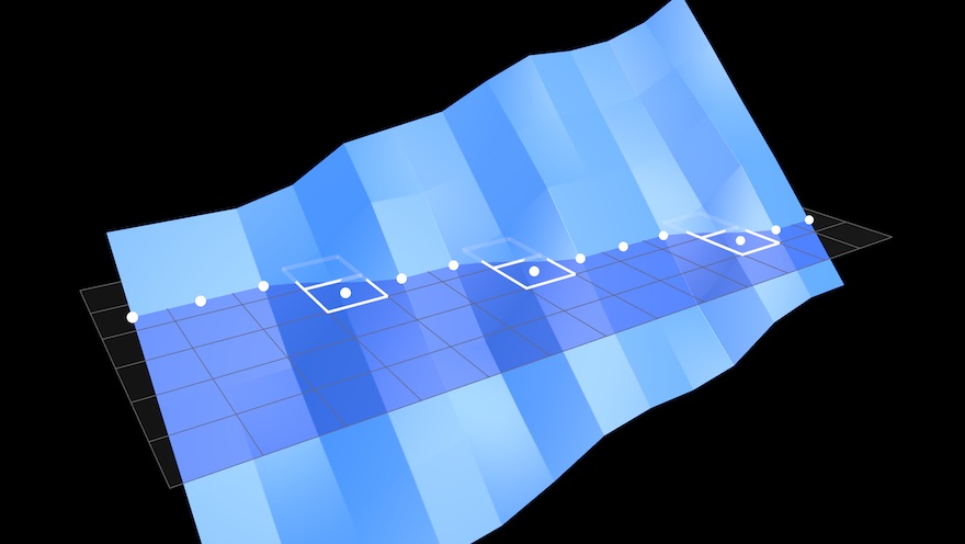
It's not obvious that you can change a signal's spectrum just by re-ordering its values over space/time, but this is easy to illustrate.
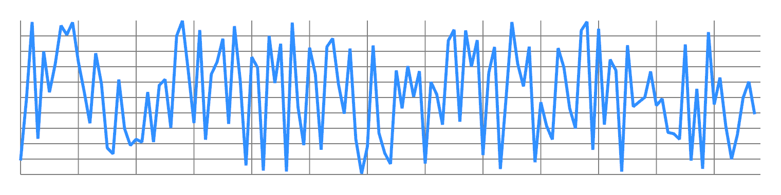
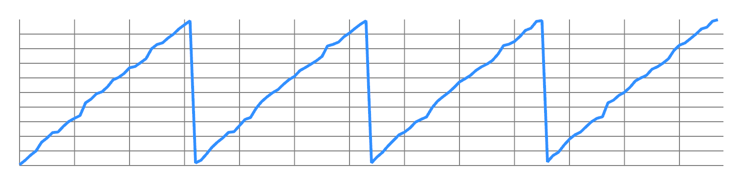
Take any finite 1D signal, and order its values from lowest to highest. You will get some kind of ramp, approximating a sawtooth wave. This concentrates most of the energy in the first non-DC frequency:
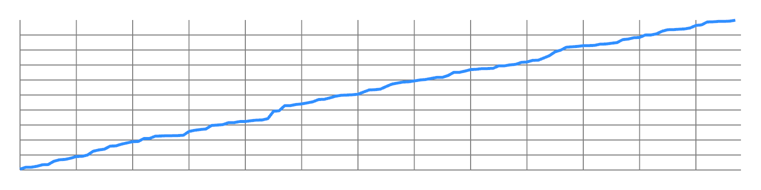
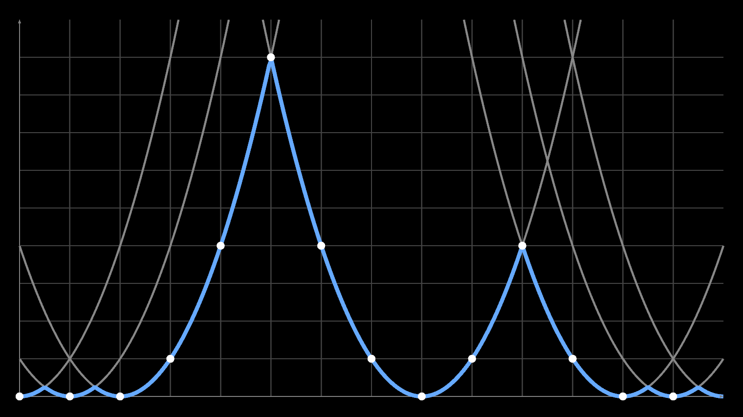
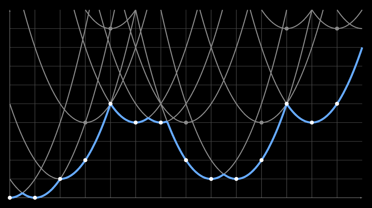
Now split the odd values from the even values, and concatenate them. You will now have two ramps, with twice the frequency:
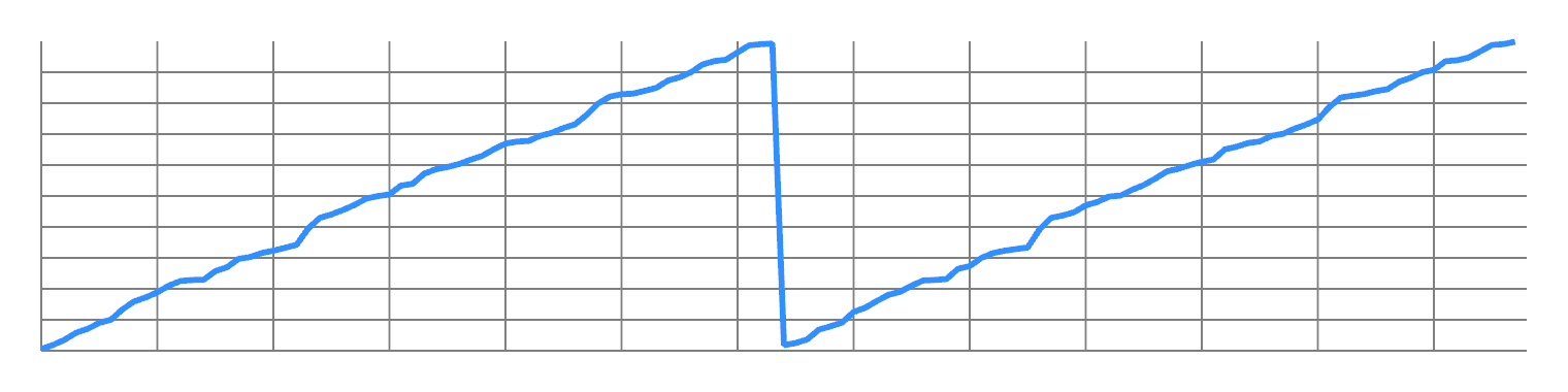
You can repeat this to double the frequency all the way up to Nyquist. So you have a lot of design freedom to transfer energy from one frequency to another.
In fact the Fourier transform has the property that energy in the time and frequency domain is conserved:
$$ \int_{-\infty}^\infty |f(x)|^2 \, dx = \int_{-\infty}^\infty |\widehat{f}(\xi)|^2 \, d\xi $$
This means the sum of $ |\mathrm{spectrum}_k|^2 $ remains constant over pixel swaps. We then design a target curve, e.g. a high-pass cosine:
$$ \mathrm{target}_k = \frac{1 - \cos \frac{k \pi}{n} }{2} $$
This can be fit and compared to the current noise spectrum to get the error to minimize.
However, I don't measure the error in energy $ |\mathrm{spectrum}_k|^2 $ but in amplitude $ |\mathrm{spectrum}_k| $. I normalize the spectrum and the target into distributions, and take the L2 norm of the difference, i.e. a sqrt of the sum of squared errors:
$$ \mathrm{error}_k = \frac{\mathrm{target}_k}{||\mathbf{target}||} - \frac{|\mathrm{spectrum}_k|}{||\mathbf{spectrum}||} $$ $$ \mathrm{loss}^2 = ||\mathbf{error}||^2 $$
This keeps the math simple, but also helps target the noise in the ~zero part of the spectrum. Otherwise, deviations near zero would count for less than deviations around one.

Go Banana
So I tried it.
With a lot of patience, you can make 2D blue noise images up to 256x256 on a single thread. A naive random search with an FFT for every iteration is not fast, but computers are.
Making a 64x64x16 with this is possible, but it's certainly like watching paint dry. It's the same number of pixels as 256x256, but with an extra dimension worth of FFTs that need to be churned.
Still, it works and you can also make 3D STBN with the spatial and temporal curves controlled independently:


Converged spectra
I built command-line scripts for this, with a bunch of quality of life things. If you're going to sit around waiting for numbers to go by, you have a lot of time for this...
- Save and load byte/float-exact state to a .png, save parameters to .json
- Save a bunch of debug viz as extra .pngs with every snapshot
- Auto-save state periodically during runs
- Measure and show rate of convergence every N seconds, with smoothing
- Validate the histogram before saving to detect bugs and avoid corrupting expensive runs
I could fire up a couple of workers to start churning, while continuing to develop the code liberally with new variations. I could also stop and restart workers with new heuristics, continuing where it left off.

Protip: you can write C in JavaScript
Drunk with power, I tried various sizes and curves, which created... okay noise. Each has the exact same uniform distribution so it's difficult to judge other than comparing to other output, or earlier versions of itself.
To address this, I visualized the blurred result, using a [1 4 6 4 1] kernel as my base line. After adjusting levels, structure was visible:

Semi-converged

Blurred
The resulting spectra show what's actually going on:

Semi-converged

Blurred
The main component is the expected ring of bandpass noise, the 2D equivalent of ringing. But in between there is also a ton of redder noise, in the lower frequencies, which all remains after a blur. This noise is as strong as the ring.
So while it's easy to make a blue-ish noise pattern that looks okay at first glance, there is a vast gap between having a noise floor and not having one. So I kept iterating:


It takes a very long time, but if you wait, all those little specks will slowly twinkle out, until quantization starts to get in the way, with a loss of about 1/255 per pixel (0.0039).
Semi converged

Fully converged
The effect on the blurred output is remarkable. All the large scale structure disappears, as you'd expect from spectra, leaving only the bandpass ringing. That goes away with a strong enough blur, or a large enough dark zone.
The visual difference between the two is slight, but nevertheless, the difference is significant and pervasive when amplified:
Semi converged

Fully converged

Difference

Final spectrum
I tried a few indigo noise curves, with different % of the curve zero. The resulting noise is all extremely equal, even after a blur and amplify. The only visible noise left is bandpass, and the noise floor is so low it may as well not be there.
As you make the black exclusion zone bigger, the noise gets concentrated in the edges and corners. It becomes a bit more linear and squarish, a contender for violet noise. This is basically a smooth evolution towards a pure pixel checkboard in the limit. Using more than 50% zero seems inadvisable for this reason:

Time domain

Frequency domain
At this point the idea was validated, but it was dog slow. Can it be done faster?
Spatially Sparse
An FFT scales like O(N log N). When you are dealing with images and volumes, that N is actually an N² or N³ in practice.
The early phase of the search is the easiest to speed up, because you can find a good swap for any pixel with barely any tries. There is no point in being clever. Each sub-region is very non-uniform, and its spectrum nearly white. Placing pixels roughly by the right location is plenty good enough.
You might try splitting a large volume into separate blocks, and optimize each block separately. That wouldn't work, because all the boundaries remain fully white. Overlapping doesn't fix this, because they will actively create new seams. I tried it.
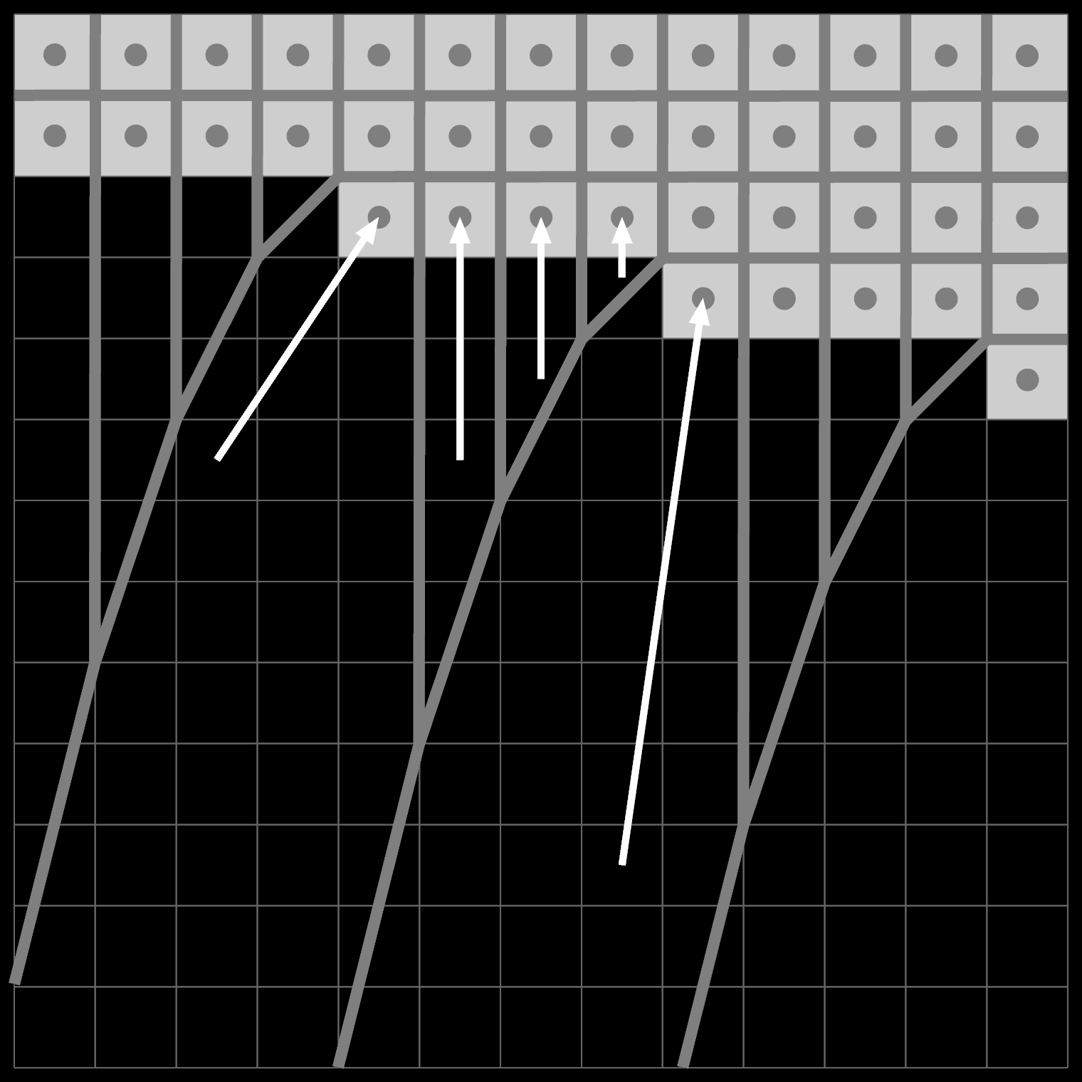
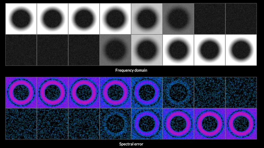
What does work is a windowed scoring strategy. It avoids a full FFT for the entire volume, and only scores each NxN or NxNxN region around each swapped point, with N-sized FFTs in each dimension. This is enormously faster and can rapidly dissolve larger volumes of white noise into approximate blue even with e.g. N = 8 or N = 16. Eventually it stops improving and you need to bump the range or switch to a global optimizer.
Here's the progression from white noise, to when sparse 16x16 gives up, followed by some additional 64x64:

Time domain

Frequency domain

Time domain

Frequency domain

Time domain

Frequency domain
A naive solution does not work well however. This is because the spectrum of a subregion does not match the spectrum of the whole.
The Fourier transform assumes each signal is periodic. If you take a random subregion and forcibly repeat it, its new spectrum will have aliasing artifacts. This would cause you to consistently misjudge swaps.
To fix this, you need to window the signal in the space/time-domain. This forces it to start and end at 0, and eliminates the effect of non-matching boundaries on the scoring. I used a smoothStep window because it's cheap, and haven't needed to try anything else:

16x16 windowed data
$$ w(t) = 1 - (3|t|^2 - 2|t|^3) , t=-1..1 $$
This still alters the spectrum, but in a predictable way. A time-domain window is a convolution in the frequency domain. You don't actually have a choice here: not using a window is mathematically equivalent to using a very bad window. It's effectively a box filter covering the cut-out area inside the larger volume, which causes spectral ringing.
The effect of the chosen window on the target spectrum can be modeled via convolution of their spectral magnitudes:
$$ \mathbf{target}' = |\mathbf{target}| \circledast |\mathcal{F}(\mathbf{window})| $$
This can be done via the time domain as:
$$ \mathbf{target}' = \mathcal{F}(\mathcal{F}^{-1}(|\mathbf{target}|) \cdot \mathcal{F}^{-1}(|\mathcal{F}(\mathbf{window})|)) $$
Note that the forward/inverse Fourier pairs are not redundant, as there is an absolute value operator in between. This discards the phase component of the window, which is irrelevant.
Curiously, while it is important to window the noise data, it isn't very important to window the target. The effect of the spectral convolution is small, amounting to a small blur, and the extra error is random and absorbed by the smooth scoring function.
The resulting local loss tracks the global loss function pretty closely. It massively speeds up the search in larger volumes, because the large FFT is the bottleneck. But it stops working well before anything resembling convergence in the frequency-domain. It does not make true blue noise, only a lookalike.
The overall problem is still that we can't tell good swaps from bad swaps without trying them and verifying.
Sleight of Frequency
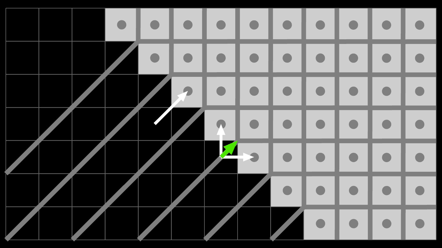
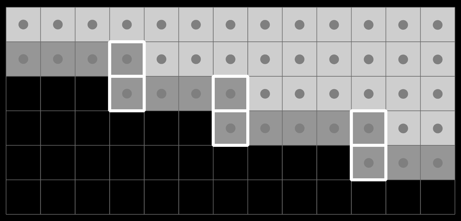
So, let's characterize the effect of a pixel swap.
Given a signal [A B C D E F G H], let's swap C and F.
Swapping the two values is the same as adding F - C = Δ to C, and subtracting that same delta from F. That is, you add the vector:
V = [0 0 Δ 0 0 -Δ 0 0]This remains true if you apply a Fourier transform and do it in the frequency domain.
To best understand this, you need to develop some intuition around FFTs of Dirac deltas.
Consider the short filter kernel [1 4 6 4 1]. It's a little known fact, but you can actually sight-read its frequency spectrum directly off the coefficients, because the filter is symmetrical. I will teach you.
The extremes are easy:
- The DC amplitude is the sum 1 + 4 + 6 + 4 + 1 = 16
- The Nyquist amplitude is the modulated sum 1 - 4 + 6 - 4 + 1 = 0
So we already know it's an 'ideal' lowpass filter, which reduces the Nyquist signal +1, -1, +1, -1, ... to exactly zero. It also has 16x DC gain.
Now all the other frequencies.
First, remember the Fourier transform works in symmetric ways. Every statement "____ in the time domain = ____ in the frequency domain" is still true if you swap the words time and frequency. This has lead to the grotesquely named sub-field of cepstral processing where you have quefrencies and vawes, and it kinda feels like you're having a stroke. The cepstral convolution filter from earlier is called a lifter.
Usually cepstral processing is applied to the real magnitude of the spectrum, i.e. $ |\mathrm{spectrum}| $, instead of its true complex value. This is a coward move.
So, decompose the kernel into symmetric pairs:
[· · 6 · ·]
[· 4 · 4 ·]
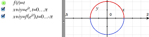
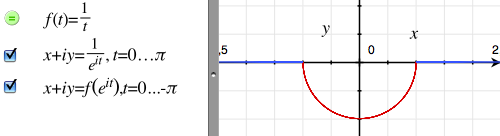
[1 · · · 1]All but the first row is a pair of real Dirac deltas in the time domain. Such a row is normally what you get when you Fourier transform a cosine, i.e.:
$$ \cos \omega = \frac{\mathrm{e}^{i\omega} + \mathrm{e}^{-i\omega}}{2} $$
A cosine in time is a pair of Dirac deltas in the frequency domain. The phase of a (real) cosine is zero, so both its deltas are real.
Now flip it around. The Fourier transform of a pair [x 0 0 ... 0 0 x] is a real cosine in frequency space. Must be true. Each new pair adds a new higher cosine on top of the existing spectrum. For the central [... 0 0 x 0 0 ...] we add a DC term. It's just a Fourier transform in the other direction:
|FFT([1 4 6 4 1])| =

  [· · 6 · ·] => 6
  [· 4 · 4 ·] => 8 cos(ɷ)
  [1 · · · 1] => 2 cos(2ɷ)

 = |6 + 8 cos(ɷ) + 2 cos(2ɷ)|
Normally you have to use the z-transform to analyze a digital filter. But the above is a shortcut. FFTs and inverse FFTs do have opposite phase, but that doesn't matter here because cos(ɷ) = cos(-ɷ).
This works for the symmetric-even case too: you offset the frequencies by half a band, ɷ/2, and there is no DC term in the middle:
|FFT([1 3 3 1])| =

  [· 3 3 ·] => 6 cos(ɷ/2)
  [1 · · 1] => 2 cos(3ɷ/2)

 = |6 cos(ɷ/2) + 2 cos(3ɷ/2)|
So, symmetric filters have spectra that are made up of regular cosines. Now you know.
For the purpose of this trick, we centered the filter around $ t = 0 $. FFTs are typically aligned to array index 0. The difference between the two is however just phase, so it can be disregarded.
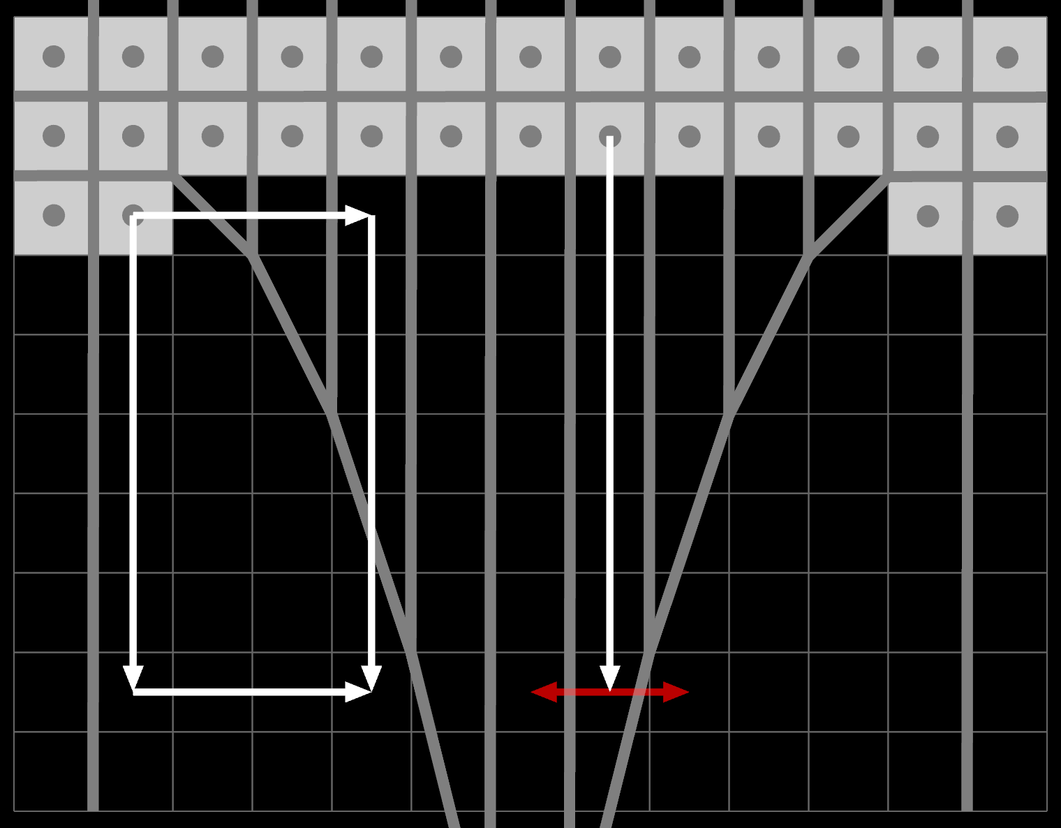
What about the delta vector [0 0 Δ 0 0 -Δ 0 0]? It's not symmetric, so we have to decompose it:
V1 = [· · · · · Δ · ·]
V2 = [· · Δ · · · · ·]

V = V2 - V1
Each is now an unpaired Dirac delta. Each vector's Fourier transform is a complex wave $ Δ \cdot \mathrm{e}^{-i \omega k} $ in the frequency domain (the k'th quefrency). It lacks the usual complementary oppositely twisting wave $ Δ \cdot \mathrm{e}^{i \omega k} $, so it's not real-valued. It has constant magnitude Δ and varying phase:
FFT(V1) = [ΔΔΔΔΔΔΔΔ]
FFT(V2) = [ΔΔΔΔΔΔΔΔ]
These are vawes.
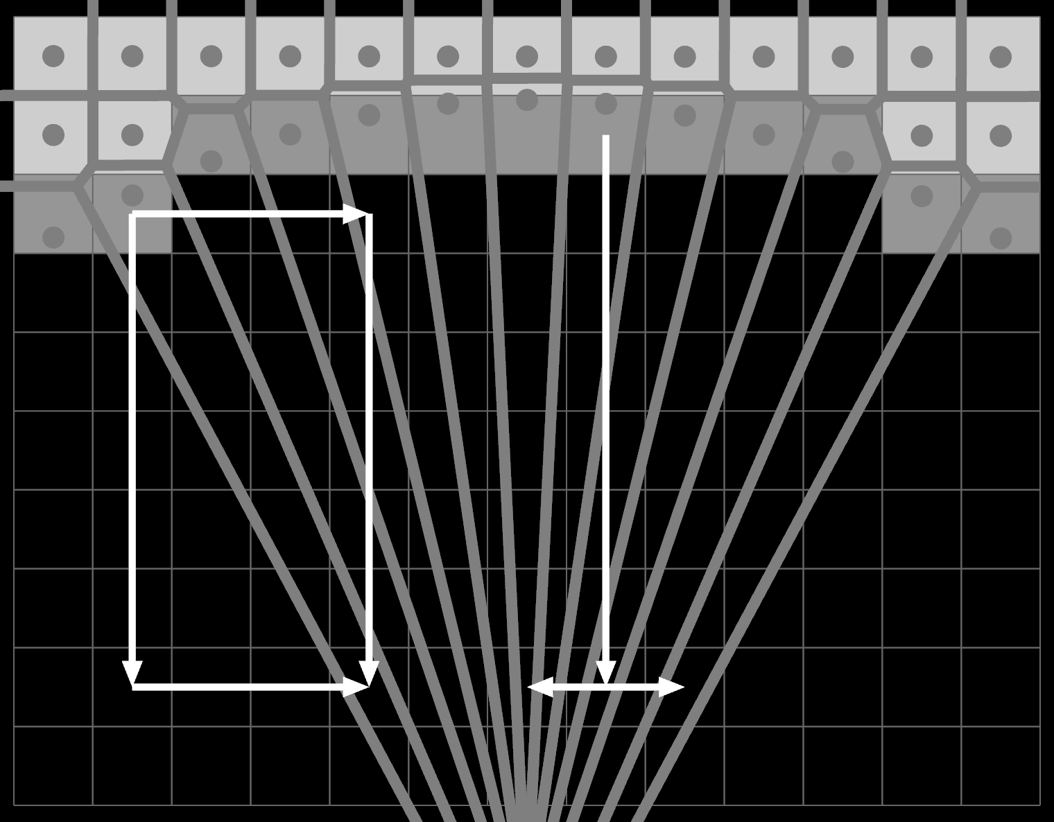
The effect of a swap is still just to add FFT(V), aka FFT(V2) - FFT(V1) to the (complex) spectrum. The effect is to transfer energy between all the bands simultaneously. Hence, FFT(V1) and FFT(V2) function as a source and destination mask for the transfer.
However, 'mask' is the wrong word, because the magnitude of $ \mathrm{e}^{i \omega k} $ is always 1. It doesn't have varying amplitude, only varying phase. -FFT(V1) and FFT(V2) define the complex direction in which to add/subtract energy.
When added together their phases interfere constructively or destructively, resulting in an amplitude that varies between 0 and 2Δ: an actual mask. The resulting phase will be halfway between the two, as it's the sum of two equal-length complex numbers.
FFT(V) = [·ΔΔΔΔΔΔΔ]For any given pixel A and its delta FFT(V1), it can pair up with other pixels B to form N-1 different interference masks FFT(V2) - FFT(V1). There are N(N-1)/2 unique interference masks, if you account for (A,B) (B,A) symmetry.
Worth pointing out, the FFT of the first index:
FFT([Δ 0 0 0 0 0 0 0]) = [Δ Δ Δ Δ Δ Δ Δ Δ]This is the DC quefrency, and the fourier symmetry continues to work. Moving values in time causes the vawe's quefrency to change in the frequency domain. This is the upside-down version of how moving energy to another frequency band causes the wave's frequency to change in the time domain.
What's the Gradient, Kenneth?
Using vectors as masks... shifting energy in directions... this means gradient descent, no?
Well.
It's indeed possible to calculate the derivative of your loss function as a function of input pixel brightness, with the usual bag of automatic differentiation/backprop tricks. You can also do it numerically.
But, this doesn't help you directly because the only way you can act on that per-pixel gradient is by swapping a pair of pixels. You need to find two quefrencies FFT(V1) and FFT(V2) which interfere in exactly the right way to decrease the loss function across all bad frequencies simultaneously, while leaving the good ones untouched. Even if the gradient were to help you pick a good starting pixel, that still leaves the problem of finding a good partner.
There are still O(N²) possible pairs to choose from, and the entire spectrum changes a little bit on every swap. Which means new FFTs to analyze it.
Random greedy search is actually tricky to beat in practice. Whatever extra work you spend on getting better samples translates into less samples tried per second. e.g. Taking a best-of-3 approach is worse than just trying 3 swaps in a row. Swaps are almost always orthogonal.
But random() still samples unevenly because it's white noise. If only we had.... oh wait. Indeed if you already have blue noise of the right size, you can use that to mildly speed up the search for more. Use it as a random permutation to drive sampling, with some inevitable whitening over time to keep it fresh. You can't however use the noise you're generating to accelerate its own search, because the two are highly correlated.
What's really going on is all a consequence of the loss function.
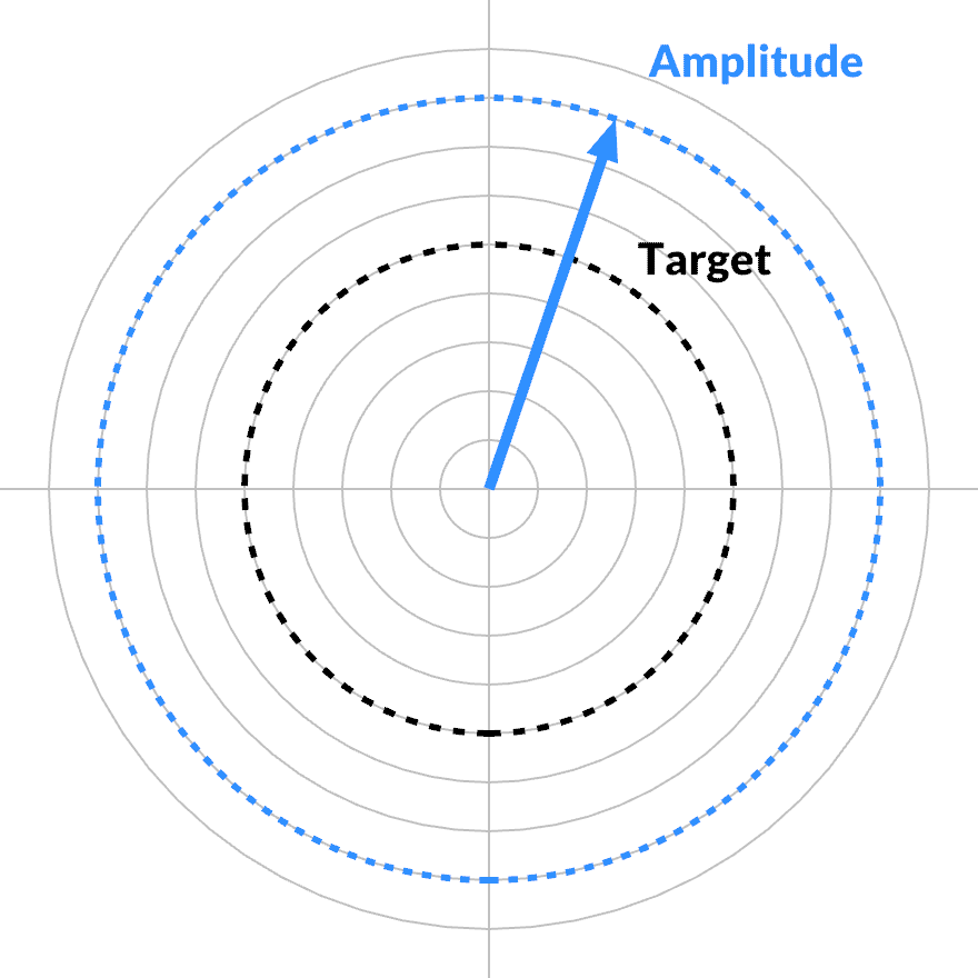
Given any particular frequency band, the loss function is only affected when its magnitude changes. Its phase can change arbitrarily, rolling around without friction. The complex gradient must point in the radial direction. In the tangential direction, the partial derivative is zero.
The value of a given interference mask FFT(V1) - FFT(V2) for a given frequency is also complex-valued. It can be projected onto the current phase, and split into its radial and tangential component with a dot product.
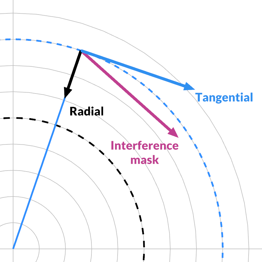
The interference mask has a dual action. As we saw, its magnitude varies between 0 and 2Δ, as a function of the two indices k1 and k2. This creates a window that is independent of the specific state or data. It defines a smooth 'hash' from the interference of two quefrency bands.
But its phase adds an additional selection effect: whether the interference in the mask is aligned with the current band's phase: this determines the split between radial and tangential. This defines a smooth phase 'hash' on top. It cycles at the average of the two quefrencies, i.e. a different, third one.
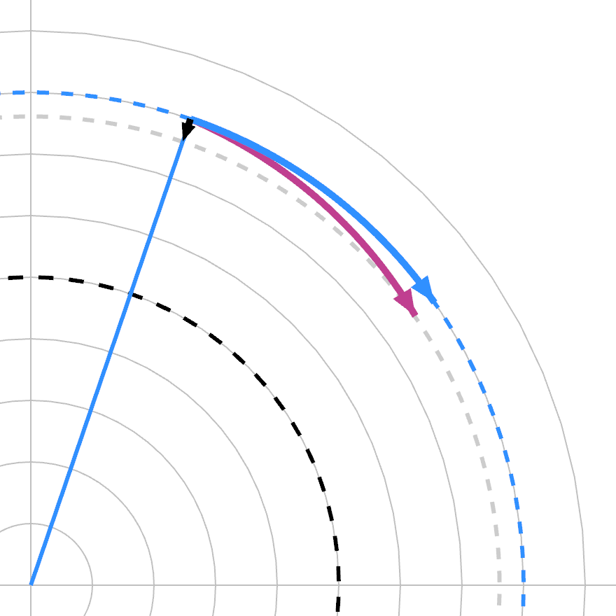
Energy is only added/subtracted if both hashes are non-zero. If the phase hash is zero, the frequency band only turns. This does not affect loss, but changes how each mask will affect it in the future. This then determines how it is coupled to other bands when you perform a particular swap.
Note that this is only true differentially: for a finite swap, the curvature of the complex domain comes into play.
The loss function is actually a hyper-cylindrical skate bowl you can ride around. Just the movement of all the bands is tied together.
Frequency bands with significant error may 'random walk' freely clockwise or counterclockwise when subjected to swaps. A band can therefor drift until it gets a turn where its phase is in alignment with enough similar bands, where the swap makes them all descend along the local gradient, enough to counter any negative effects elsewhere.
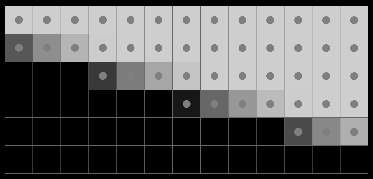
In the time domain, each frequency band is a wave that oscillates between -1...1: it 'owns' some of the value of each pixel, but there are places where its weight is ~zero (the knots).
So when a band shifts phase, it changes how much of the energy of each pixel it 'owns'. This allows each band to 'scan' different parts of the noise in the time domain. In order to fix a particular peak or dent in the frequency spectrum, the search must rotate that band's phase so it strongly owns any defect in the noise, and then perform a swap to fix that defect.
Thus, my mental model of this is not actually disconnected pixel swapping.
It's more like one of those Myst puzzles where flipping a switch flips some of the neighbors too. You press one pair of buttons at a time. It's a giant haunted dimmer switch.
We're dealing with complex amplitudes, not real values, so the light also has a color. Mechanically it's like a slot machine, with dials that can rotate to display different sides. The cherries and bells are the color: they determine how the light gets brighter or darker. If a dial is set just right, you can use it as a /dev/null to 'dump' changes.
That's what theory predicts, but does it work? Well, here is a (blurred noise) spectrum being late-optimized. The search is trying to eliminate the left-over lower frequency noise in the middle:

Semi converged
Here's the phase difference from the late stages of search, each a good swap. Left to right shows 4 different value scales:

x2

x16

x256

x4096

x2

x16

x256

x4096
At first it looks like just a few phases are changing, but amplification reveals it's the opposite. There are several plateaus. Strongest are the bands being actively modified. Then there's the circular error area around it, where other bands are still swirling into phase. Then there's a sharp drop-off to a much weaker noise floor, present everywhere. These are the bands that are already converged.
Compare to a random bad swap:

x2

x16

x256

x4096
Now there is strong noise all over the center, and the loss immediately gets worse, as a bunch of amplitudes start shifting in the wrong direction randomly.
So it's true. Applying the swap algorithm with a spectral target naturally cycles through focusing on different parts of the target spectrum as it makes progress. This information is positionally encoded in the phases of the bands and can be 'queried' by attempting a swap.
This means the constraint of a fixed target spectrum is actually a constantly moving target in the complex domain.
Frequency bands that reach the target are locked in. Neither their magnitude nor phase changes in aggregate. The random walks of such bands must have no DC component... they must be complex-valued blue noise with a tiny amplitude.
Knowing this doesn't help directly, but it does explain why the search is so hard. Because the interference masks function like hashes, there is no simple pattern to how positions map to errors in the spectrum. And once you get close to the target, finding new good swaps is equivalent to digging out information encoded deep in the phase domain, with O(N²) interference masks to choose from.
Gradient Sampling
As I was trying to optimize for evenness after blur, it occurred to me to simply try selecting bright or dark spots in the blurred after-image.
This is the situation where frequency bands are in coupled alignment: the error in the spectrum has a relatively concentrated footprint in the time domain. But, this heuristic merely picks out good swaps that are already 'lined up' so to speak. It only works as a low-hanging fruit sampler, with rapidly diminishing returns.
Next I used the gradient in the frequency domain.
The gradient points towards increasing loss, which is the sum of squared distance $ (…)^2 $. So the slope is $ 2(…) $, proportional to distance to the goal:
$$ |\mathrm{gradient}_k| = 2 \cdot \left( \frac{|\mathrm{spectrum}_k|}{||\mathbf{spectrum}||} - \frac{\mathrm{target}_k}{||\mathbf{target}||} \right) $$
It's radial, so its phase matches the spectrum itself:
$$ \mathrm{gradient}_k = \mathrm{|gradient_k|} \cdot \left(1 ∠ \mathrm{arg}(\mathrm{spectrum}_k) \right) $$
Eagle-eyed readers may notice the sqrt part of the L2 norm is missing here. It's only there for normalization, and in fact, you generally want a gradient that decreases the closer you get to the target. It acts as a natural stabilizer, forming a convex optimization problem.
You can transport this gradient backwards by applying an inverse FFT. Usually derivatives and FFTs don't commute, but that's only when you are deriving in the same dimension as the FFT. The partial derivative here is neither over time nor frequency, but by signal value.
The resulting time-domain gradient tells you how fast the (squared) loss would change if a given pixel changed. The sign tells you whether it needs to become lighter or darker. In theory, a pixel with a large gradient can enable larger score improvements per step.
It says little about what's a suitable pixel to pair with though. You can infer that a pixel needs to be paired with one that is brighter or darker, but not how much. The gradient only applies differentially. It involves two pixels, so it will cause interference between the two deltas, and also with the signal's own phase.
The time-domain gradient does change slowly after every swap—mainly the swapping pixels—so this only needs to add an extra IFFT every N swap attempts, reusing it in between.
I tried this in two ways. One was to bias random sampling towards points with the largest gradients. This barely did anything, when applied to one or both pixels.
Then I tried going down the list in order, and this worked better. I tried a bunch of heuristics here, like adding a retry until paired, and a 'dud' tracker to reject known unpairable pixels. It did lead to some minor gains in successful sample selection. But beating random was still not a sure bet in all cases, because it comes at the cost of ordering and tracking all pixels to sample them.
All in all, it was quite mystifying.
Pair Analysis
Hence I analyzed all possible swaps (A,B) inside one 64x64 image at different stages of convergence, for 1024 pixels A (25% of total).
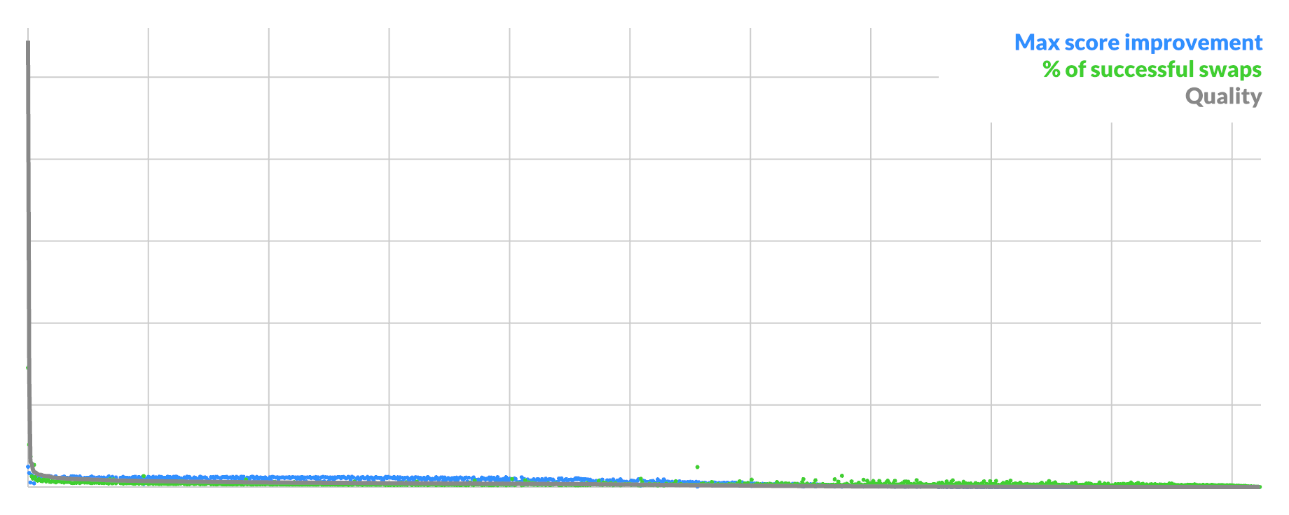
The result was quite illuminating. There are 2 indicators of a pixel's suitability for swapping:
- % of all possible swaps (A,_) that are good
- score improvement of best possible swap (A,B)
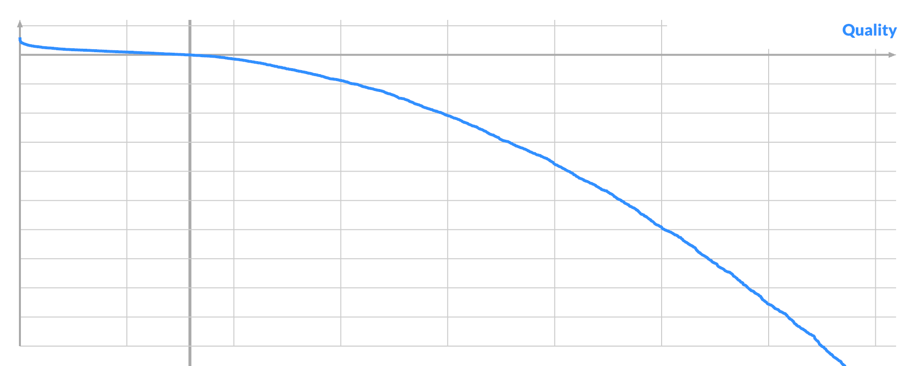
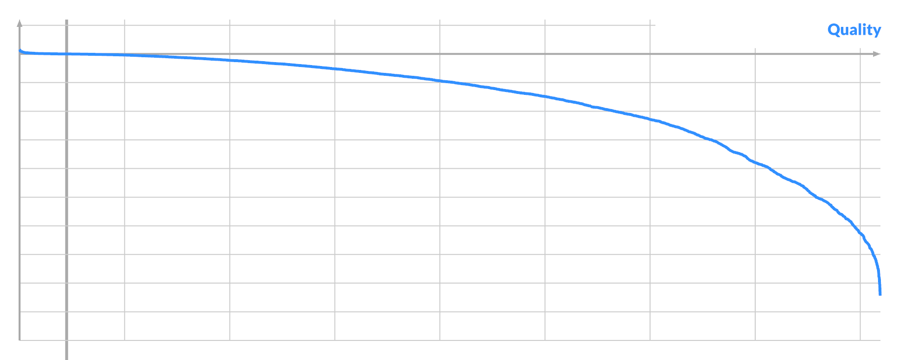
They are highly correlated, and you can take the geometric average to get a single quality score to order by:
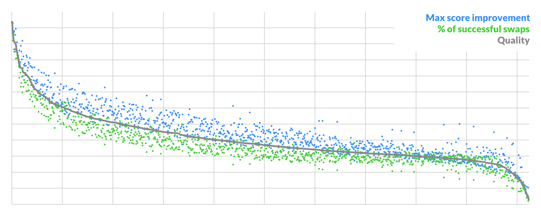
The curve shows that the best possible candidates are rare, with a sharp drop-off at the start. Here the average candidate is ~1/3rd as good as the best, though every pixel is pairable. This represents the typical situation when you have unconverged blue-ish noise.
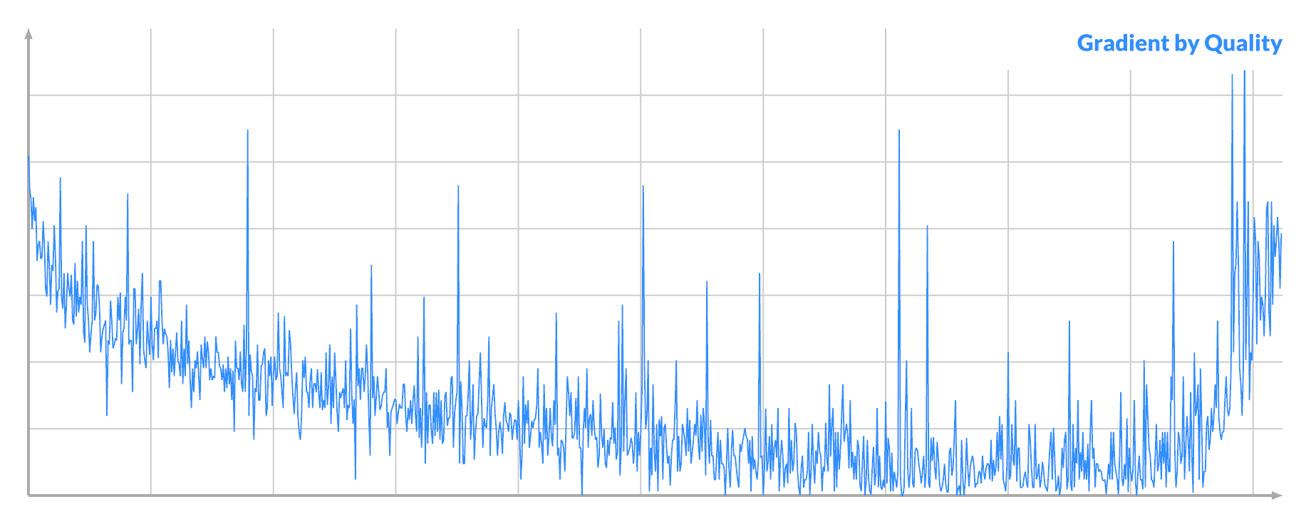
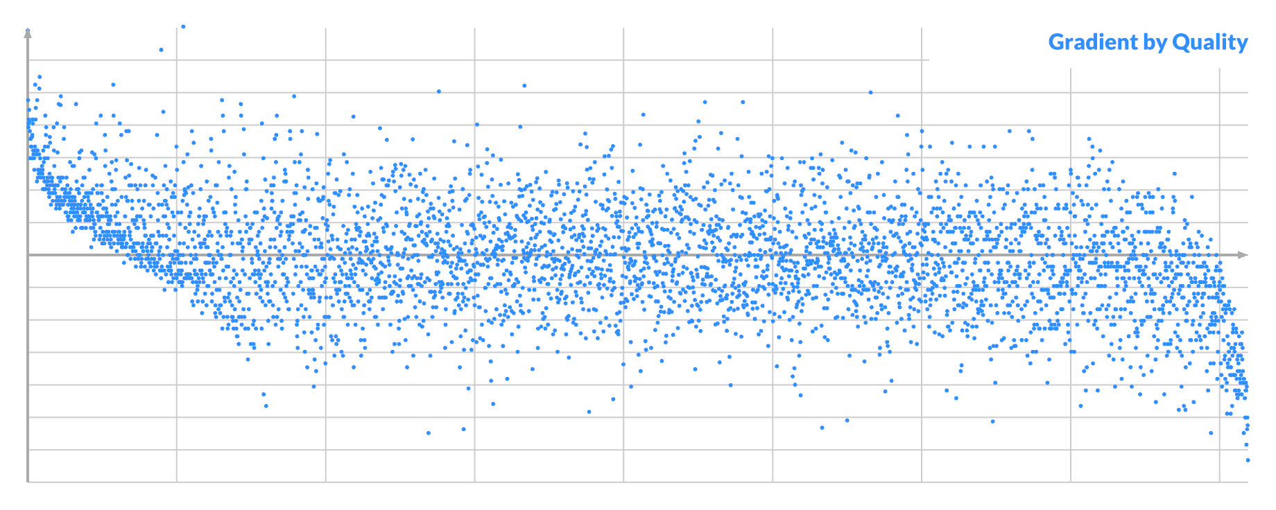
Order all pixels by their (signed) gradient, and plot the quality:
The distribution seems biased towards the ends. A larger absolute gradient at A can indeed lead to both better scores and higher % of good swaps.
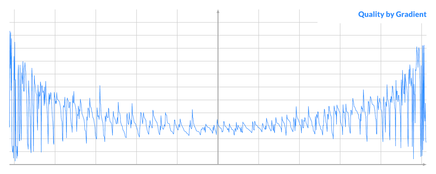
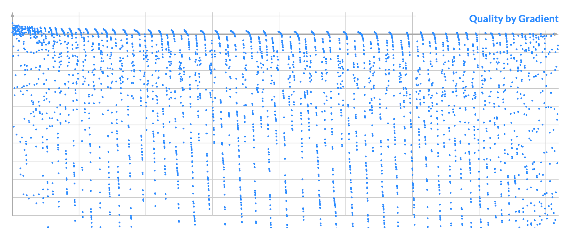
Notice that it's also noisier at the ends, where it dips below the middle. If you order pixels by their quality, and then plot the absolute gradient, you see:
Selecting for large gradient at A will select both the best and the worst possible pixels A. This implies that there are pixels in the noise that are very significant, but are nevertheless currently 'unfixable'. This corresponds to the 'focus' described earlier.
By drawing from the 'top', I was mining the imbalance between the good/left and bad/right distribution. Selecting for a vanishing gradient would instead select the average-to-bad pixels A.
I investigated one instance of each: very good, average or very bad pixel A. I tried every possible swap (A, B) and plotted the curve again. Here the quality is just the actual score improvement:
The three scenarios have similar curves, with the bulk of swaps being negative. Only a tiny bit of the curve is sticking out positive, even in the best case. The potential benefit of a good swap is dwarfed by the potential harm of bad swaps. The main difference is just how many positive swaps there are, if any.
So let's focus on the positive case, where you can see best.
You can order by score, and plot the gradient of all the pixels B, to see another correlation.
It looks kinda promising. Here the sign matters, with left and right being different. If the gradient of pixel A is the opposite sign, then this graph is mirrored.
But if you order by (signed) gradient and plot the score, you see the real problem, caused by the noise:
The good samples are mixed freely among the bad ones, with only a very weak trend downward. This explains why sampling improvements based purely on gradient for pixel B are impossible.
You can see what's going on if you plot Δv, the difference in value between A and B:
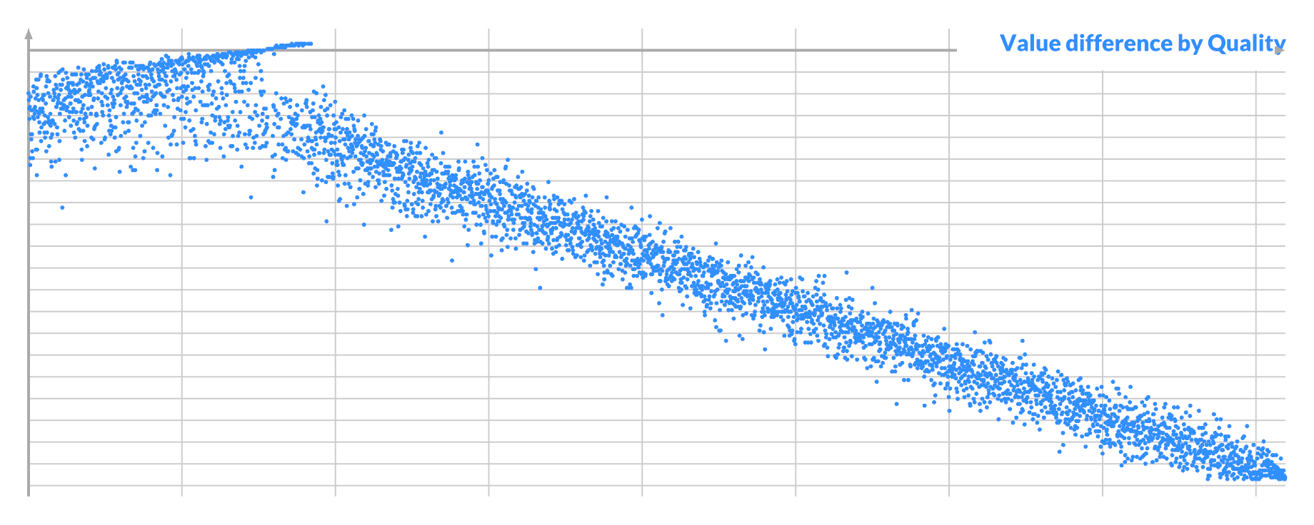
For a given pixel A, all the good swaps have a similar value for B, which is not unexpected. Its mean is the ideal value for A, but there is a lot of variance. In this case pixel A is nearly white, so it is brighter than almost every other pixel B.
If you now plot Δv * -gradient, you see a clue on the left:
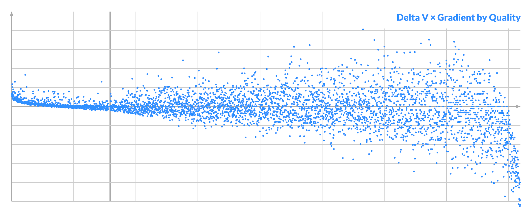
Almost all of the successful swaps have a small but positive value.
This represents what we already knew: the gradient's sign tells you if a pixel should be brighter or darker. If Δv has the opposite sign, the chances of a successful swap are slim.
Ideally both pixels 'face' the right way, so the swap is beneficial on both ends. But only the combined effect on the loss matters: i.e. Δv * Δgradient < 0.
It's only true differentially so it can misfire. But compared to blind sampling of pairs, it's easily 5-10x better and faster, racing towards the tougher parts of the search.
What's more... while this test is just binary, I found that any effort spent on trying to further prioritize swaps by the magnitude of the gradient is entirely wasted. Maximizing Δv * Δgradient by repeated sampling is counterproductive, because it selects more bad candidates on the right. Minimizing Δv * Δgradient creates more successful swaps on the left, but lowers the average improvement per step so the convergence is net slower. Anything more sophisticated incurs too much computation to be worth it.
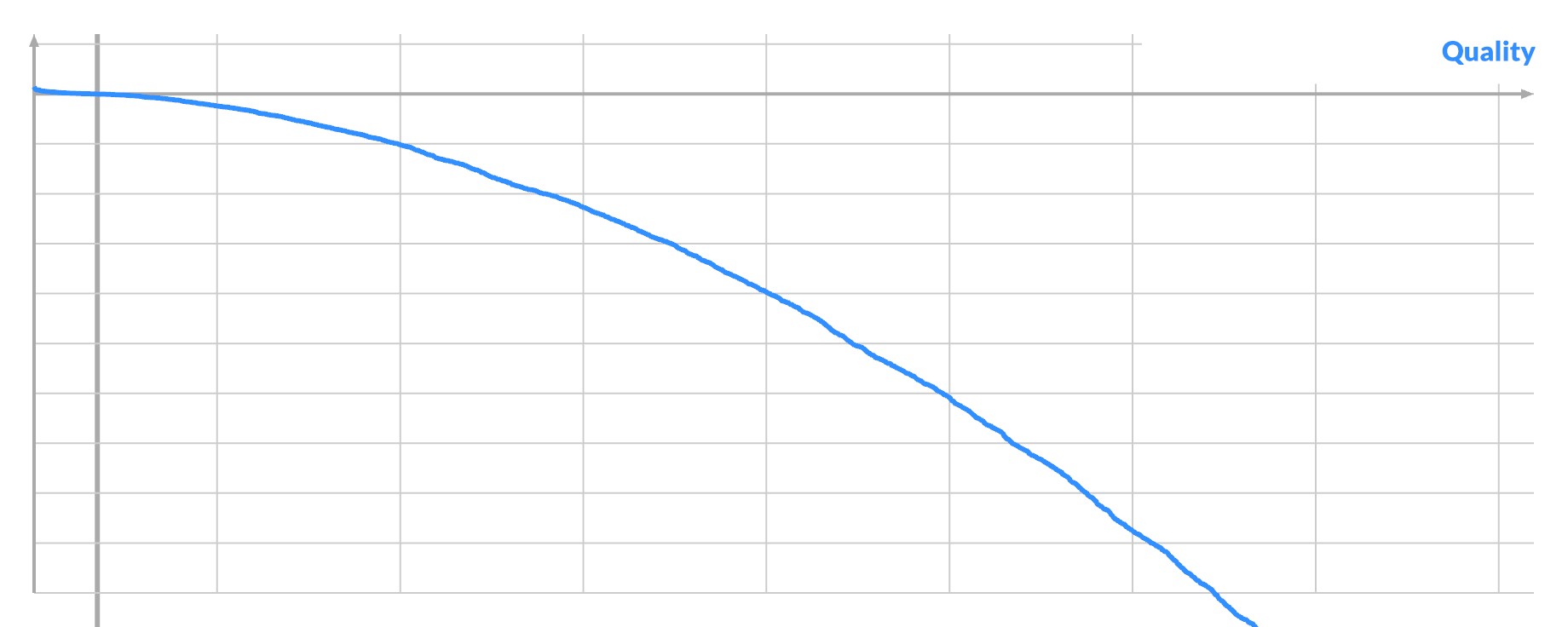
It does have a limit. This is what it looks like when an image is practically fully converged:
Eventually you reach the point where there are only a handful of swaps with any real benefit, while the rest is just shaving off a few bits of loss at a time. It devolves back to pure random selection, only skipping the coin flip for the gradient. It is likely that more targeted heuristics can still work here.
The gradient also works in the early stages. As it barely changes over successive swaps, this leads to a different kind of sparse mode. Instead of scoring only a subset of pixels, simply score multiple swaps as a group over time, without re-scoring intermediate states. This lowers the success rate roughly by a power (e.g. 0.8 -> 0.64), but cuts the number of FFTs by a constant factor (e.g. 1/2). Early on this trade-off can be worth it.
Even faster: don't score steps at all. In the very early stage, you can easily get up to 80-90% successful swaps just by filtering on values and gradients. If you just swap a bunch in a row, there is a very good chance you will still end up better than before.
It works better than sparse scoring: using the gradient of your true objective approximately works better than using an approximate objective exactly.
The latter will miss the true goal by design, while the former continually re-aims itself to the destination despite inaccuracy.
Obviously you can mix and match techniques, and gradient + sparse is actually a winning combo. I've only scratched the surface here.
Warp Speed
Time to address the elephant in the room. If the main bottleneck is an FFT, wouldn't this work better on a GPU?
The answer to that is an unsurprising yes, at least for large sizes where the overhead of async dispatch is negligible. However, it would have been endlessly more cumbersome to discover all of the above based on a GPU implementation, where I can't just log intermediate values to a console.
After checking everything, I pulled out my bag of tricks and ported it to Use.GPU. As a result, the algorithm runs entirely on the GPU, and provides live visualization of the entire process. It requires a WebGPU-enabled browser, which in practice means Chrome on Windows or Mac, or a dev build elsewhere.

I haven't particularly optimized this—the FFT is vanilla textbook—but it works. It provides an easy ~8x speed up on an M1 Mac on beefier target sizes. With a desktop GPU, 128x128x32 and larger become very feasible.
It lacks a few goodies from the scripts, and only does gradient + optional sparse. You can however freely exchange PNGs between the CPU and GPU version via drag and drop, as long as the settings match.
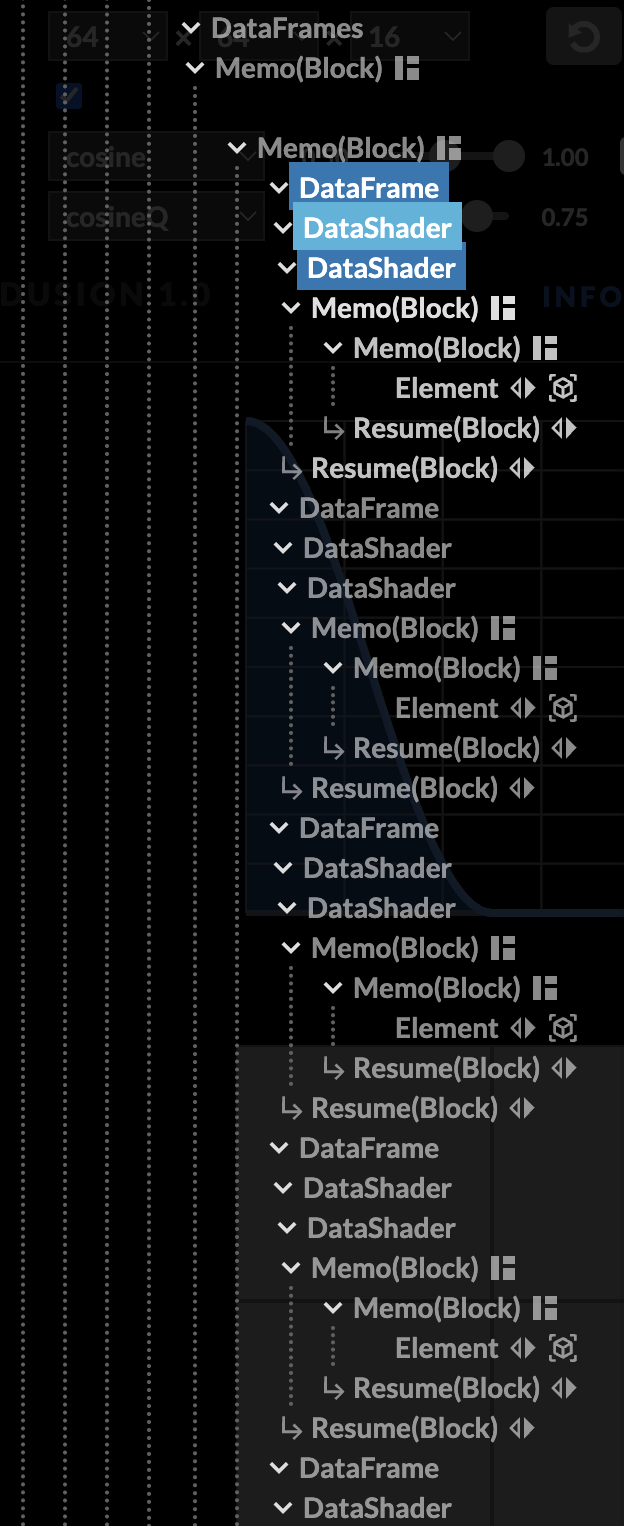
Layout components
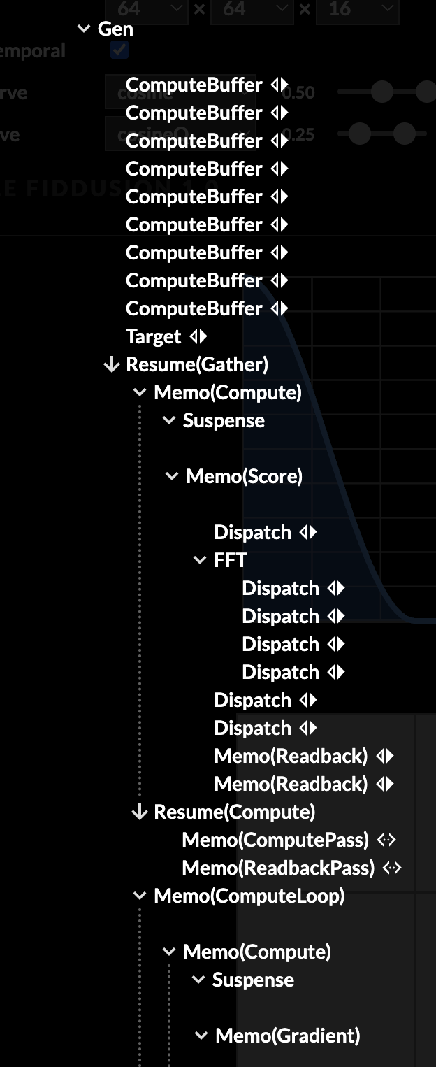
Compute components
Worth pointing out: this visualization is built using Use.GPU's HTML-like layout system. I can put div-like blocks inside a flex box wrapper, and put text beside it... while at the same time using raw WGSL shaders as the contents of those divs. These visualization shaders sample and colorize the algorithm state on the fly, with no CPU-side involvement other than a static dispatch. The only GPU -> CPU readback is for the stats in the corner, which are classic React and real HTML, along with the rest of the controls.
I can then build an <FFT> component and drop it inside an async <ComputeLoop>, and it does exactly what it should. The rest is just a handful of <Dispatch> elements and the ordinary headache of writing compute shaders. <Suspense> ensures all the shaders are compiled before dispatching.
While running, the bulk of the tree is inert, with only a handful of reducers triggering on a loop, causing a mere 7 live components to update per frame. The compute dispatch fights with the normal rendering for GPU resources, so there is an auto-batching mechanism that aims for approximately 30-60 FPS.
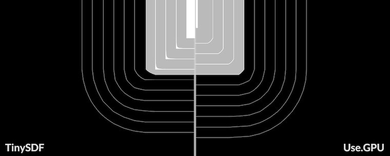
The display is fully anti-aliased, including the pixelized data. I'm using the usual per-pixel SDF trickery to do this... it's applied as a generic wrapper shader for any UV-based sampler.
It's a good showcase that Use.GPU really is React-for-GPUs with less hassle, but still with all the goodies. It bypasses most of the browser once the canvas gets going, and it isn't just for UI: you can express async compute just fine with the right component design. The robust layout and vector plotting capabilities are just extra on top.
I won't claim it's the world's most elegant abstraction, because it's far too pragmatic for that. But I simply don't know any other programming environment where I could even try something like this and not get bogged down in GPU binding hell, or have to round-trip everything back to the CPU.
* * *
So there you have it: blue and indigo noise à la carte.
What I find most interesting is that the problem of generating noise in the time domain has been recast into shaping and denoising a spectrum in the frequency domain. It starts as white noise, and gets turned into a pre-designed picture. You do so by swapping pixels in the other domain. The state for this process is kept in the phase channel, which is not directly relevant to the problem, but drifts into alignment over time.
Hence I called it Stable Fiddusion. If you swap the two domains, you're turning noise into a picture by swapping frequency bands without changing their values. It would result in a complex-valued picture, whose magnitude is the target, and whose phase encodes the progress of the convergence process.
This is approximately what you get when you add a hidden layer to a diffusion model.
What I also find interesting is that the notion of swaps naturally creates a space that is O(N²) big with only N samples of actual data. Viewed from the perspective of a single step, every pair (A,B) corresponds to a unique information mask in the frequency domain that extracts a unique delta from the same data. There is redundancy, of course, but the nature of the Fourier transform smears it out into one big superposition. When you do multiple swaps, the space grows, but not quite that fast: any permutation of the same non-overlapping swaps is equivalent. There is also a notion of entanglement: frequency bands / pixels are linked together to move as a whole by default, but parts will diffuse into being locked in place.
Phase is kind of the bugbear of the DSP world. Everyone knows it's there, but they prefer not to talk about it unless its content is neat and simple. Hopefully by now you have a better appreciation of the true nature of a Fourier transform. Not just as a spectrum for a real-valued signal, but as a complex-valued transform of a complex-valued input.
During a swap run, the phase channel continuously looks like noise, but is actually highly structured when queried with the right quefrency hashes. I wonder what other things look like that, when you flip them around.
More: