<?xml version="1.0" encoding="utf-8"?>
<feed xmlns="http://www.w3.org/2005/Atom">

  <title><![CDATA[Acko.net]]></title>
  <link href="https://acko.net/atom.xml" rel="self"/>
  <link href="https://acko.net/"/>
  <updated>2026-03-05T12:10:39+01:00</updated>
  <id>https://acko.net</id>
  <author>
    <name><![CDATA[Steven Wittens]]></name>
    
  </author>

  
  <entry>
    <title type="html"><![CDATA[To Infinity… And Beyond!]]></title>
    <link href="https://acko.net/blog/to-infinity-and-beyond/"/>
    <updated>2013-01-28T00:00:00+01:00</updated>
    <id>https://acko.net/blog/to-infinity-and-beyond</id>
    <content type="html"><![CDATA[<script type="text/x-mathjax-config">
MathJax.Hub.Config({
  "HTML-CSS": { availableFonts: ["TeX"] },
  extensions: ["tex2jax.js"],
  jax: ["input/TeX","output/HTML-CSS"],
  tex2jax: {inlineMath: [["$","$"],["\\(","\\)"]]},
});
</script>

<script type="text/javascript" src="https://cdn.mathjax.org/mathjax/latest/MathJax.js?config=TeX-AMS_HTML.js">
</script>

<script type="text/javascript">
// <!--
window.MathJax && MathJax.Hub.Queue(["Typeset",MathJax.Hub]);
Acko.queue(function () { Acko.Fallback.warnWebGL(); });
// -->
</script>

<div class="g8 i2"><div class="pad">

<h2 class="sub">Exploring the outer limits</h2>

</div></div>

<div class="c"></div>

<div class="g12"><div class="pad">

<blockquote class="m2">
  <em class="big">“It is known that there are an infinite number of worlds, simply because there is an infinite amount of space for them to be in. However, not every one of them is inhabited. Therefore, there must be a finite number of inhabited worlds.<br /><br />
Any finite number divided by infinity is as near to nothing as makes no odds, so the average population of all the planets in the universe can be said to be zero. From this it follows that the population of the whole universe is also zero, and that any people you may meet from time to time are merely the products of a deranged imagination.”</em>
  <div class="tr m1">– <a href="http://en.wikipedia.org/wiki/The_Restaurant_at_the_End_of_the_Universe">The Restaurant at the End of the Universe</a>, Douglas Adams</div>
</blockquote>

</div></div>

<div class="g8 i2 m2"><div class="pad">

<p>If there's one thing mathematicians have a love-hate relationship with, it has to be <em>infinity</em>. It's the ultimate tease: it beckons us to come closer, but never allows us anywhere near it. No matter how far we travel to impress it, infinity remains disinterested, equally distant from everything: infinitely far!</p>

<p class="tc math">$$ 0 &lt; 1 &lt; 2 &lt; 3 &lt; … &lt; \infty $$</p>

<p>Yet infinity is not just desirable, it is absolutely necessary. All over mathematics, we find problems for which no finite amount of steps will help resolve them. Without infinity, we wouldn't have real numbers, for starters. That's a problem: our circles aren't round anymore (no <a href="http://en.wikipedia.org/wiki/Pi">$ π $ and $ \tau $</a>) and our exponentials stop growing right (no <a href="http://en.wikipedia.org/wiki/E_(mathematical_constant)">$ e $</a>). We can throw out all of our triangles too: most of their sides have exploded.</p>

</div></div>

<div class="g7">
  <p><a href="http://www.loc.gov/pictures/resource/ggbain.16674/"><img src="/files/infinity-and-beyond/steel-bridge-loc.jpg" title="Cape Cod Canal, Buzzard's Bay, 1910" alt="Steel Railroad Bridge,  Cape Cod Canal, Buzzard's Bay, 1910" /></a></p>
  <p class="tc">A steel railroad bridge with a 1200 ton counter-weight.<br />Completed in 1910. Source: <a href="http://www.loc.gov/pictures/resource/ggbain.16674/">Library of Congress</a>.</p></div>

<div class="g5"><div class="pad">

<p class="math">We like infinity because it helps avoid all that. In fact even when things are not infinite, we often prefer to pretend they are—we do geometry in infinitely big planes, because then we don't have to care about where the edges are.</p>

<p class="math">Now, suppose we want to analyze a steel beam, because we're trying to figure out if our proposed bridge will stay up. If we want to model reality accurately, that means simulating each individual particle, every atom in the beam. Each has its own place and pushes and pulls on others nearby.</p>

<p class="math">But even just $ 40 $ grams of pure iron contains <a href="http://www.wolframalpha.com/input/?i=40g+of+iron+in+atoms">$ 4.31 \cdot 10^{23} $ atoms</a>. That's an inordinate amount of things to keep track of for just <a href="http://www.wolframalpha.com/input/?i=%281+teaspoon%29+%2F+%2840g+%2F+density+of+iron%29">1 teaspoon of iron</a>.</p>

</div></div>

<aside class="g6">
  <p class="mt0"><iframe class="mathbox square autosize" src="/files/infinity-and-beyond/mb-1-austenite.html"></iframe></p>
  <p class="tc">The crystal structure of 32 iron atoms in the hot <a href="http://en.wikipedia.org/wiki/Austenite">austenite</a> phase.<br />If your steel looks like this, your bridge is on fire.</p>
</aside>

<aside class="g6">
  <p class="mt0"><iframe class="mathbox square autosize" src="/files/infinity-and-beyond/mb-2-cube.html"></iframe></p>
  <p class="tc">A chunk of solid, mathematical iron.</p>
</aside>

<div class="g8 i2"><div class="pad">
<p>Instead, we pretend the steel is solid throughout. Rather than being composed of atoms with gaps in between, it's made of some unknown, filled in material with a certain density, expressed e.g. as <em>grams per cubic centimetre</em>. Given any shape, we can determine its volume, and hence its total mass, and go from there. That's much simpler than counting and keeping track of individual atoms, right?</p>

<p>Unfortunately, that's not quite true.</p>

<h2>The Shortest Disappearing Trick Ever</h2>
<p class="math">Like all choices in mathematics, this one has consequences we cannot avoid. Our beam's density is <em>mass per volume</em>. Individual points in space have zero volume. That would mean that at any given point inside the beam, the amount of mass there is $ 0 $. How can a beam that is entirely composed of nothing be solid and have a non-zero mass?</p>

<p class="tc">
<iframe class="mathbox fit" src="/files/infinity-and-beyond/mb-3-empty-cube.html" height="250"></iframe><br /><em>Bam! No more iron anywhere.</em></p>

<p>While Douglas Adams was being deliberately obtuse, there's a kernel of truth there, which is a genuine paradox: what exactly is the mass of every atom in our situation?</p>

<p class="math">To make our beam solid and continuous, we had to shrink every atom down to an infinitely small point. To compensate, we had to create infinitely many of them. Dividing the finite mass of the beam between an infinite amount of atoms should result in $ 0 $ mass per atom. Yet all these masses still have to add up to the total mass of the beam. This suggests $ 0 + 0 + 0 + … &gt; 0 $, which seems impossible.</p>

<p class="math">If the mass of every atom were not $ 0 $, and we have infinitely many points inside the beam, then the total mass is infinity times the atomic mass $ m $. Yet the total mass is finite. This suggests $ m + m + m + … &lt; \infty $, which also doesn't seem right.</p>

<p class="math">It seems whatever this number $ m $ is, it can't be $ 0 $ and can't be non-zero. It's definitely not infinite, we only had a finite mass to begin with. It's starting to sound like we'll have to invent a whole new set of numbers again to even find it.</p>

</div></div>

<div class="g8"><div class="pad">

<p>That's effectively what Isaac Newton and Gottfried Leibniz set in motion at the end of the 17th century, when they <a href="http://en.wikipedia.org/wiki/Leibniz–Newton_calculus_controversy">both discovered calculus independently</a>. It was without a doubt the most important discovery in mathematics and resulted in formal solutions to many problems that were previously unsolvable— our entire understanding of physics has relied on it since. Yet it took until the late 19th century for the works of Augustin Cauchy and Karl Weierstrass to pop up, which formalized the required theory of <em>convergence</em>. This allows us to describe exactly how differences can shrink down to nothing as you approach infinity. Even that wasn't enough: it was only in the 1960s when the idea of <a href="http://en.wikipedia.org/wiki/Infinitesimal">infinitesimals</a> as fully functioning numbers—the <a href="http://en.wikipedia.org/wiki/Hyperreal_number">hyperreal numbers</a>—was finally proven to be consistent enough by Abraham Robinson.</p>

<p class="math">But it goes back much further. Ancient mathematicians were aware of problems of infinity, and used many ingenious ways to approach it. For example, $ π $ was found by considering circles to be infinite-sided polygons. <a href="http://en.wikipedia.org/wiki/Archimedes%27_use_of_infinitesimals">Archimedes' work</a> is likely the earliest use of <em>indivisibles</em>, using them to imagine tiny mechanical levers and find a shape's center of mass. He's better known for running naked through the streets shouting <a href="http://en.wikipedia.org/wiki/Eureka_(word)#Archimedes">Eureka!</a> though.</p>

<p class="math">That it took so long shows that this is not an easy problem. The proofs involved are elaborate and meticulous, all the way back. They have to be, in order to nail down something as tricky as infinity. As a result, students generally learn calculus through the simplified methods of Newton and Leibniz, rather than the most mathematically correct interpretation. We're taught to mix notations from 4 different centuries together, and everyone's just supposed to connect the dots on their own. Except the trail of important questions along the way is now overgrown with jungle.</p>

</div></div>

<aside class="g4">
  <p><img class="pad" src="/files/infinity-and-beyond/principia.png" /></p>
  <p class="tc">A diagram from Isaac Newton's <a href="http://en.wikipedia.org/wiki/Philosophiæ_Naturalis_Principia_Mathematica">Philosophiæ Naturalis Principia Mathematica</a> (1687) about finding area under a smooth curve.</p></aside>

<div class="g8 i2"><div class="pad">
  
<p>Still, it shows that even if we don't understand the whole picture, we can get a lot done. This article is in no way a formal introduction to infinitesimals. Rather, it's a demonstration of why we might need them.</p>
  
<p class="math">What is happening when we shrink atoms down to points? Why does it make shapes solid yet seemingly hollow? Is it ever meaningful to write $ x = \infty $? Is there only one infinity, or are there many different kinds?</p>

<p>To answer that, we first have to go back to even simpler times, to Ancient Greece, and start with the works of Zeno.</p>

<h2>Achilles and the Tortoise</h2>

<p><a href="http://en.wikipedia.org/wiki/Zeno_of_Elea">Zeno of Elea</a> was one of the first mathematicians to pose these sorts of questions, effectively trolling mathematics for the next two millennia. He lived in the 5th century BC in southern Italy, although only second-hand references survive. In his series of paradoxes, he examines the nature of equality, distance, continuity, of time itself.</p>

<p>Because it's the ancient times, our mathematical knowledge is limited. We know about zero, but we're still struggling with the idea of nothing. We've run into negative numbers, but they're clearly absurd and imaginary, unlike the positive numbers we find in geometry. We also know about fractions and ratios, but square roots still confuse us, even though our temples stay up.</p>

</div></div>

<div class="wide slideshow full">

  <div class="iframe c">
    <iframe src="/files/infinity-and-beyond/mb-4-achilles.html" class="mathbox paged autosize" height="320"></iframe>
  </div>

  <div class="steps">

    <div class="step">
      <p>So the story goes: the tortoise challenges Achilles to a footrace.</p>
    </div>

    <div class="step">
      <p>
        "If you give me a head start," it says, "any start at all, you can never win.".<br />
        Achilles laughs and decides to be a good sport: he'll only run twice as fast as the tortoise.
      </p>
    </div>

    <div class="step">
      <p>
        The tortoise explains: "If you want to pass me, first you have to move to where I am. By the time you get there, I'll have walked ahead a little bit."
      </p>
    </div>

    <div class="step">
      <p>
        "While you cross the next distance, I will move yet again. No matter how many times you try to catch up, I'll always be some small distance ahead. Therefor, you cannot beat me."
      </p>
    </div>

    <div class="step">
      <p>Achilles realizes that talking tortoises are not a sign of positive mental health, so he decides to find a wall to run into instead. It will either confirm the theory, or end the pain.
      </p>
    </div>

    <div class="step">
      <p>
        See, the race is actually unnecessary, because the problem remains the same.<br />In order to reach the wall, Achilles first has to cross half the way there.
      </p>
    </div>
    
    <div class="step">
      <p>Then he has to go half that distance again, and again. No matter how many times he repeats this, there will always be some distance left. So if Achilles can't cross this distance in a finite amount of steps, why is he wearing that stupid helmet?
      </p>
    </div>

    <div class="step">
      <div class="extra bottom" data-delay="2.4" data-hold="2" data-align-y=".55"><big>$$ … $$</big></div>
      <p>
        The <em>distance travelled</em> forms a never ending <span class="orangered">sequence of expanding sums</span>.<br />We have to examine the entire sequence, rather than individual numbers in it.
      </p>
    </div>

    <div class="step">
      <p class="math">
        By definition, the <span class="orangered">distance travelled</span> and <span class="gold">distance to the wall</span> always add up to $ 1 $. So one simple way to resolve this conundrum is to say: <em>Well yes, it's going to take you infinitely long to glue all those pieces together, but only because you already spent an infinite amount of time chopping them up!</em><br />
        But that's not a very mathematically satisfying answer. Let's try something else.
      </p>
    </div>

    <div class="step">
      <p class="math">
        The distance to the wall is always equal to the last step taken. We know that each step is half as long as the previous one, starting with $ \frac{1}{2} $. Therefor, the distance to the wall must decrease exponentially: $ \frac{1}{2}, \frac{1}{4}, \frac{1}{8}, \frac{1}{16}, … $, getting closer to zero with every step.
      </p>
    </div>

    <div class="step">
      <p class="math">
        But why can we say that this gap effectively closes to zero after 'infinity steps'? The number that we're building up is $ \frac{1}{2} + \frac{1}{4} + \frac{1}{8} + \frac{1}{16} + … \,$
      </p>
    </div>
    
    <div class="step">
      <p class="math">
        We know our sum will never exceed $ 1 $, as there is only $ 1 $ unit of distance being divided. This means $ \frac{1}{2} + \frac{1}{4} + \frac{1}{8} + \frac{1}{16} + … \leq 1 $, which eliminates every number past the surface of the wall—but not the surface itself.
      </p>
    </div>

    <div class="step">
      <p class="math">
        Suppose we presume $ \frac{1}{2} + \frac{1}{4} + \frac{1}{8} + \frac{1}{16} + … &lt; 1 $ and hence that this number lies some tiny distance <em>in front of the wall</em>.
      </p>
    </div>

    <div class="step">
      <p class="math">
        Well in that case, all we need to do is zoom in far enough, and we'll see our sequence jump past it after a certain finite number of steps.
      </p>
    </div>

    <div class="step">
      <p class="math">
        If we try to move it <span class="gold">closer to the wall</span>, the same thing happens. This number simply cannot be less than $ 1 $. Therefor $ \frac{1}{2} + \frac{1}{4} + \frac{1}{8} + \frac{1}{16} + … \geq 1 $
      </p>
    </div>

    <div class="step">
      <p class="math">
        The only place $ \frac{1}{2} + \frac{1}{4} + \frac{1}{8} + \frac{1}{16} + … \, $ can be is exactly $ 0 $ units away from $ 1 $. If two numbers have zero distance between them, then they are equal.
      </p>
    </div>

    <div class="step">
      <div class="extra bottom" data-delay="4.6" data-hold="1" data-align-y=".55"><big>$$ … $$</big></div>
      <p class="math">
        What we've actually done here is applied the principle of <em>limits</em>: we've defined a procedure of steps that lets us narrow down <span class="gold">the interval</span> where the infinite sum might be. The lower bound is the sequence of sums itself: it only increases towards $ 1 $, never decreases. For the upper bound, we established no sum could exceed $ 1 $. Therefor the interval must shrink to nothing, and the sequence <em>converges</em>.
      </p>
    </div>

    <div class="step">
      <div class="extra"><big><big>
        $$ \lim_{n \to +\infty} x_n = \mathop{\class{no-outline}{►\hspace{-2pt}►}}_{\infty\hspace{2pt}} x_n $$
      </big></big></div>
      <p class="math">
        The purpose of a limit is then to act as a supercharged fast-forward button. It lets us avoid the infinite amount of work required to complete sums like $ \frac{1}{2} + \frac{1}{4} + \frac{1}{8} + \frac{1}{16} + … $ and simply <em>skip to the end</em>. To do so, we have to step back, spot the pattern, and pin down where it ends. So limits allow us to literally reach the unreachable. But in fact, you already knew that.
      </p>
    </div>

    <div class="step">
      <div class="extra top right" data-delay="2.4" data-align-x="1.25" data-align-y=".5">$$ \frac{2}{3} = 0.66666… $$</div>
      <div class="extra bottom" data-delay="2.4" data-align-y=".58">$$ 0.6 + 0.06 + 0.006 + …\hspace{2pt} $$</div>
      <p class="math">
        As soon as you learned to divide, you found $ 2 \div 3 = 0.666… = 0.6 + 0.06 + 0.006 + …\hspace{2pt} $ <br />Even in primary school the opportunity to examine infinity is there. Rather than tackle it head on, it's simply noted and filed. Eight years later it's regurgitated in the form of cryptic <em>epsilon-delta definitions</em>.</p>
    </div>

    <div class="step">
      <div class="extra bottom" data-delay="1.6" data-hold="1" data-align-y="1.1">
        $$ 1 - 1 + 1 - 1 + 1 … $$<br />
      </div>
      <p class="math">
        But then there's those pesky consequences again. By allowing the idea of infinity, we can invent an entire zoo of paradoxical things. For example, imagine a lamp that's switched on ($1$) and off ($0$) at intervals that decrease by a factor of two: <em>on</em> for $ \frac{1}{2} $ second, <em>off</em> for $ \frac{1}{4} s $, <em>on</em> for $ \frac{1}{8} s $, <em>off</em> for $ \frac{1}{16} s $, …<br />After $ 1\,s $, when the switch has been flipped an infinite amount of times, is the lamp on or off?
      </p>
    </div>

    <div class="step">
      <div class="extra bottom" data-align-y="1.1">
        <br /><br />
        <small><small>
        <br />
        $$ (1 - 1) + (1 - 1) + (1 - 1) + … = 0 \,? $$
        </small></small>
      </div>
      <div class="extra bottom" data-align-y="1.1">
        <br /><br />
        <small><small>
        <br />
        <br /><br />
        $$ 1 + (-1 + 1) + (-1 + 1) + … = 1 \,? $$
        </small></small>
      </div>
      <p class="math">
        Another way to put this is that the lamp's state at $ 1\,s $ is the result of the infinite sum $ 1 - 1 + 1 - 1 + … $ <br />Intuitively we might say each pair of $ +1 $ and $ -1 $ should cancel out and make the entire sum equal to $ 0 $. <br />But we can pair them the other way, leading to $ 1 $ instead. It can't be both.
      </p>
    </div>

    <div class="step">
      <p class="math">
        If we zoom in, it's obvious that no matter how close we get to $ 1\,s $, the lamp's state keeps switching. Therefor it's meaningless to attempt to 'fast forward' to the end, and the limit does not exist. At $ 1\,s $ the lamp is neither on nor off: it's undefined. This infinite sum <em>does not converge</em>.
      </p>
    </div>

    <div class="step">
      <p class="math">
        But actually, we overcomplicated things. Thanks to the power of limits, we can ask a simpler, equivalent question. Given a lamp that switches on and off <em>every second</em>, what is its state at infinity? The answer's the same: it never settles.
      </p>
    </div>

  </div>
  
</div>

<div class="c"></div>

<div class="g8 i2"><div class="pad">
  
  <p class="math">Limits are the first tool in our belt for tackling infinity. Given a sequence described by countable steps, we can attempt to extend it not just to the end of the world, but literally forever. If this works we end up with a finite value. If not, the limit is undefined. A limit can be equal to $ \infty $, but that's just shorthand for <em>the sequence has no upper bound</em>. Negative infinity means no lower bound.</p>

<h2>Breaking Away From Rationality</h2>
  
  <p>Until now we've only encountered fractions, that is, <em>rational numbers</em>. Each of our sums was made of fractions. The limit, if it existed, was also a rational number. We don't know whether this was just a coincidence.</p>
  
  <p class="math">It might seem implausible that a sequence of numbers that is 100% rational and converges, can approach a limit that isn't rational at all. Yet we've already seen similar discrepancies. In our first sequence, every partial sum was <em>less than</em> $ 1 $. Meanwhile the limit of the sum was <em>equal to</em> $ 1 $. Clearly, the limit does not have to share all the properties of its originating sequence.</p>
  
  <p>We also haven't solved our original problem: we've only chopped things up into infinitely many <em>finite pieces</em>. How do we get to <em>infinitely small pieces</em>? To answer that, we need to go looking for <em>continuity</em>.</p>
  
  <p>Generally, continuity is defined by what it is and what its properties are: a noticeable lack of holes, and no paradoxical values. But that's putting the cart before the horse. First, we have to show which holes we're trying to plug.</p>
  
</div></div>

<div class="wide slideshow full">

  <div class="iframe c">
    <iframe src="/files/infinity-and-beyond/mb-5-continuity.html" class="mathbox paged autosize" height="320"></iframe>
  </div>

  <div class="steps">

    <div class="step">
      <p>Let's imagine the <em>rational numbers</em>.</p>
    </div>

    <div class="step">
      <p>Actually, hold on. Is this really a line? The integers certainly weren't connected.</p>
    </div>

    <div class="step">
      <p class="math">Rather than assume anything, we're going to attempt to visualize all the rational numbers. We'll start with the <span class="blue">numbers between $ 0 $ and $ 1 $</span>.</p>
    </div>

    <div class="step">
      <div class="extra bottom"><big>$$ \class{blue}{\frac{0 + 1}{2}} $$</big></div>
      <p class="math">Between any two numbers, we can find a new number in between: their average. This leads to $ \frac{1}{2} $.</p>
    </div>

    <div class="step">
      <div class="extra bottom"><big>$$ \frac{a + b}{2} $$</big></div>
      <p>By repeatedly taking averages, we keep finding new numbers, filling up the interval.</p>
    </div>

    <div class="step">
      <p>If we separate out every step, we get a <em>binary tree</em>.</p>
    </div>

    <div class="step">
      <p class="math">You can think of this as a map of all the fractions of $ 2^n $. Given any such fraction, say <big>$ \frac{13}{32} = \frac{13}{2^5} $</big>, there is a unique path of lefts and rights that leads directly to it. At least, as long as it lies between $ 0 $ and $ 1 $.</p>
    </div>
  
    <div class="step">
      <p class="math">
      Note that the graph resembles a fractal and that the distance to the top edge is divided in half with every step. But we only ever explore a finite amount of steps. Therefor, we are not taking a limit and we'll never actually touch the edge. 
      </p>
    </div>

    <div class="step">
      <div class="extra left" data-hold="1">$$ \frac{2 \cdot a + b}{3} $$</div>
      <div class="extra right" data-hold="1">$$ \frac{a + 2 \cdot b}{3} $$</div>
      <p class="math">But we can take thirds as well, leading to fractions with a power of $ 3^n $ in their denominator.</p>
    </div>

    <div class="step">
      <p class="math">As some numbers can be reached in multiple ways, we can eliminate some lines, and end up with this graph, where every number sprouts into a three-way, <em>ternary tree</em>. Again, we have a map that gives us a unique path to any fraction of $ 3^n $ in this range, like <big>$ \frac{11}{27} = \frac{11}{3^3} $</big>.</p>
    </div>

    <div class="step">
      <div class="extra">
        $$ \frac{21}{60} = \frac{21}{2^2 \cdot 3 \cdot 5} $$
      </div>
      
      <p class="math">Because we can do this for any denominator, we can define a way to get to any rational number in a finite amount of steps. Take for example <big>$ \frac{21}{60} $</big>. We decompose its denominator into prime numbers and begin with $ 0 $ and $ 1 $ again.</p>
    </div>

    <div class="step">
      <div class="extra top edge hold3">
        <small><small>
        $$ \frac{21}{60} = \frac{21}{2^2 \cdot 3 \cdot 5} $$
        </small></small>
      </div>

      <p class="math">There is a division of $ 2^2 $, so we do two binary splits. This time, I'm repeating the previously found numbers so you can see the regular divisions more clearly. We get <span class="green">quarters</span>.</p>
    </div>

    <div class="step">
      <p class="math">The next factor is $ 3 $ so we divide into thirds once. We now have <span class="gold">twelfths</span>.</p>
    </div>

    <div class="step">
      <p class="math">For the last division we chop into fifths and get <span class="orangered">sixtieths</span>.</p>
    </div>
    
    <div class="step">
      <p class="math">$ \frac{21}{60} $ is now the <span class="orangered">21st number from the left</span>.</p>
    </div>

    <div class="step">
      <p class="math">But this means we've found a clear way to visualize <em>all</em> the rational numbers between $ 0 $ and $ 1 $: it's all the numbers we can reach by applying a finite number of binary (2), ternary (3), quinary (5) etc. divisions, for any denominator. So there's always a finite <em>gap</em> between any two rational numbers, even though there are infinitely many of them.</p>
    </div>

    <div class="step">
      <p>The rational numbers are <em>not continuous</em>. Therefor, it is more accurate to picture them as a set of tick marks than a connected number line.</p>
    </div>

    <div class="step">
      <p class="math">To find continuity then, we need to revisit one of our earlier trees. We'll pick the binary one.<br />While every fork goes two ways, we actually have a third choice at every step: we can choose to stop. That's how we get a finite path to a whole fraction of $ 2^n $.</p>
    </div>

    <div class="step">
      <p>But what if we never stop? We have to apply a limit: we try to spot a pattern and try to <span class="green">fast-forward it</span>. Note that by halving each step vertically on the graph, we've actually <em>linearized</em> each approach into a straight line which ends. Now we can <em>take limits visually</em> just by intersecting lines with the top edge.</p>
    </div>

    <div class="step">
      <p class="math">Right away we can spot two convergent limits: by always choosing either the <span class="orangered">left</span> or the <span class="green">right</span> branch, we end up at respectively $ 0 $ and $ 1 $.</p>
    </div>

    <div class="step">
      <p class="math"><span class="orangered">These</span> <span class="green">two</span> sequences both converge to $ \frac{1}{2} $. It seems that 'at infinity steps', the graph meets up with itself in the middle.</p>
    </div>

    <div class="step">
      <p class="math">But the graph is now a true fractal. So the same convergence can be found here. In fact, the graph meets up with itself anywhere there is a multiple of <big>$ \frac{1}{2^n} $</big>.</p>
    </div>
    
    <div class="step">
      <p class="math">That's pretty neat: now we can eliminate the option of stopping altogether. Instead of ending at $  \frac{5}{16} $, we can simply take <span class="purple">one additional step in either direction, followed by infinitely many opposite steps</span>. Now we're <em>only</em> considering paths that are infinitely long.</p>
    </div>

    <div class="step">
      <p class="math">But if this graph only leads to fractions of $ 2^n $, then there must be gaps between them. In the limit, the distance between any two adjacent numbers in the graph shrinks down to <em>exactly</em> $ 0 $, which suggests there are no gaps. This infinite version of the binary tree must lead to a lot more numbers than we might think.<br />
         Suppose we take a path of <span class="orangered">alternating left and right steps</span>, and extend it forever. Where do we end up?</p>
    </div>

    <div class="step">
      <p>We can apply the same principle of an <span class="gold">upper and lower bound</span>, but now we're approaching from both sides at once. Thanks to our linearization trick, the entire sequence fits snugly inside a triangle.</p>
    </div>

    <div class="step">
      <p class="math">If we zoom into the convergence at infinity, we actually end up at $ \class{orangered}{\frac{2}{3}} $.<br />
        Somehow we've managed to coax a fraction of $ 3 $ out of a perfectly regular <em>binary</em> tree.</p>
    </div>

    <div class="step">
      <p class="math">If we <span class="orangered">alternate two lefts with one right</span>, we can end up at $ \class{orangered}{\frac{4}{7}} $. This is remarkable: when we tried to visualize all the rational numbers by combining all kinds of divisions, we were overthinking it. We only needed to take <em>binary divisions</em> and repeat them infinitely with a <em>limit</em>.</p>
    </div>

    <div class="step">
      <p>Every single rational number can then be found by taking a finite amount of steps to get to a certain point, and then settling into a <em>repeating pattern of lefts and/or rights</em> all the way to infinity.</p>
    </div>

    <div class="step">
      <p class="math">If we can find numbers between $ 0 $ and $ 1 $ this way, we can apply the exact same principle to the range $ 1 $ to $ 2 $. So we can connect two of these graphs into a single graph with its tip at $ 1 $.</p>
    </div>

    <div class="step">
      <p class="math">But we can repeat it as much as we like. The full graph is not just infinitely divided, but infinitely big, in that no finite box can contain it. That means it leads to <em>every single positive rational number</em>. We can start anywhere we like. Is your mind blown yet?</p>
    </div>

    <div class="step">
      <p class="math">No? Ok. But if this works for positives, we can build a similar graph for the negatives just by mirroring it. So we now have a map of the entire rational number set. All we need to do is take <em>infinite paths that settle into a repeating pattern</em> from either a positive or a negative starting point. When we do, we find every such path leads to a rational number.<br />
        So any rational number can be found by taking an infinite stroll on one of <em>two</em> infinite binary trees.</p>
    </div>

    <div class="step">
      <p class="math">Wait, did I say two infinite trees? Sorry, I meant <em>one</em> infinitely big tree.<br />See, if we repeatedly scale up a <span class="green">fractal binary tree</span> and apply a limit to that, we end up with almost exactly the same thing. Only this time, the two downward diagonals always eventually fold back towards $ 0 $. This creates a path of <em>infinity + 1</em> steps downward. While that might not be very practical, it suggests you can ride out to the restaurant at the end of the universe, have dinner, and take a single step to get back home.</p>
    </div>

    <div class="step">
      <p class="math">Is it math, or visual poetry? It's time to bring this fellatio of the mind to its inevitable climax.</p>
    </div>
    
    <div class="step">
      <div class="extra hold2 bottom left" data-align-x=".4" data-align-y=".8">$ \class{blue}{0} $</div>
      <div class="extra hold2 bottom right" data-align-x=".4" data-align-y=".8">$ \class{green}{1} $</div>

      <div class="extra hold2 left top" data-align-x="1.0" data-align-y="0.25">$ \class{blue}{0} $</div>
      <div class="extra hold2 left top" data-align-x=".6" data-align-y="0.25">$ \class{green}{1} $</div>

      <div class="extra hold2 right top" data-align-x=".6" data-align-y="0.25">$ \class{blue}{0} $</div>
      <div class="extra hold2 right top" data-align-x="1.0" data-align-y="0.25">$ \class{green}{1} $</div>
      
      <p class="math">You may wonder, if this map is so amazing, how did we ever do without?<br />
        Let's label our branches. If we go left, we call it $ 0 $. If we go right, we call it $ 1 $.</p>
    </div>

    <div class="step">
      <div class="extra">
        $$
        \frac{5}{3} = \class{green}{11}\class{blue}{0}\hspace{2pt}\class{green}{1}\class{blue}{0}\hspace{2pt}\class{green}{1}\class{blue}{0}…
        $$
      </div>

      <p class="math">We can then identify any number by writing out the infinite path that leads there as a sequence of ones and zeroes—bits.<br /><br />But you already knew that.</p>
    </div>

    <div class="step">
      <div class="extra">
        $$
        \frac{5}{3} = \class{green}{1}.\class{green}{1}\class{blue}{0}\hspace{2pt}\class{green}{1}\class{blue}{0}\hspace{2pt}\class{green}{1}\class{blue}{0}…_2
        $$
      </div>

      <p class="math">See we've just rediscovered the binary number system. We're so used to numbers in decimal, <em>base 10</em>, we didn't notice. Yet we all learned that rational numbers consist of digits that settle into a repeating sequence, a <em>repeating pattern of turns</em>. Disallowing finite paths works the same, even in decimal: the number $ 0.95 $ can be written as $\, 0.94999…\, $, i.e. <em>take one final step in one direction, followed by infinitely many steps the other way</em>.</p>
    </div>

    <div class="step">
      <div class="extra">
        $$
        \frac{4}{5} = \class{blue}{0}.\class{green}{11}\class{blue}{00}\hspace{2pt}\class{green}{11}\class{blue}{00}…_2 
        $$
      </div>

      <p class="math">
        When we write down a number digit by digit, we're really <em>following the path to it</em> in a graph like this, dialing the number's … er … number. The rationals aren't <em>shaped</em> like a binary tree, rather, they <em>look</em> like a binary tree when viewed through the lens of binary division. Every infinite binary, ternary, quinary, etc. tree is then a different but complete perspective of the same underlying thing. We don't have <em>the</em> map, we have one of infinitely many maps.</p>
    </div>

    <div class="step">
      <div class="extra top" data-delay=".8" data-align-y=".25">
        $$
        π = \class{green}{11}.\class{blue}{00}\class{green}{1}\class{blue}{00}\class{green}{1}\class{blue}{0000}\class{green}{1}…_2
        $$
      </div>
      
      <p class="math">
       Which means we can show this graph is actually an interdimensional number portal.<br />
       See, we already know <em>where</em> the missing numbers are. Irrational numbers like $ π $ form a never-repeating sequence of digits. If we want to reach $ π $, we find it's at the end of an infinite path whose turns <em>do not repeat</em>. By allowing such paths, our map leads us straight to them. Even though it's made out of only  <em>one kind of rational number</em>: division by two.</p>
    </div>

    <div class="step">
      <div class="extra" data-delay="1.6"><big><big>
        $$
          π = \mathop{\class{no-outline}{►\hspace{-2pt}►}}_{\infty\hspace{2pt}} x_n \,?
        $$
        </big></big>
      </div>

      <p class="math">
        So now we've invented <em>real numbers</em>. How do we visualize this invention? And where does continuity come in? What we need is a procedure that generates such a non-repeating path <em>when taken to the limit</em>. Then we can figure out where the behavior at infinity comes from.
      </p>
    </div>

    <div class="step">
      <p>Because the path never settles into a pattern, we can't pin it down with a single neat triangle like before. We try something else. At every step, we can see that the <em>smallest</em> number we can still reach is found by <span class="orangered">always going left</span>. Similarly, the <em>largest</em> available number is found by <span class="green">always going right</span>. Wherever we go from here, it will be somewhere in this range.</p>
    </div>

    <div class="step">
      <p>We can set up shrinking intervals by placing such triangles along the path, forming a nested sequence.</p>
    </div>

    <div class="step">
      <div class="extra left">
        $$
          \begin{align}
            3 \leq &amp; π \leq 4 \\
            3.1 \leq &amp; π \leq 3.2 \\
            3.14 \leq &amp; π \leq 3.15 \\ 
            3.141 \leq &amp; π \leq 3.142 \\ 
            3.1415 \leq &amp; π \leq 3.1416 \\
            3.14159 \leq &amp; π \leq 3.14160 \\
          \end{align}
        $$
      </div>

      <div class="extra right">
        $$
          \begin{align}
            11_2 \leq &amp; π \leq 100_2 \\ 
            11.0_2 \leq &amp; π \leq 11.1_2 \\ 
            11.00_2 \leq &amp; π \leq 11.01_2 \\
            11.001_2 \leq &amp; π \leq 11.010_2 \\
            11.0010_2 \leq &amp; π \leq 11.0011_2 \\
            11.00100_2 \leq &amp; π \leq 11.00101_2 \\
          \end{align}
        $$
      </div>

      <p class="math">
        What we've actually done is rounded up and down at every step, to find an upper and lower bound with a certain amount of digits. This works in any number base.
      </p>
    </div>

    <div class="step">
      <p class="math">Let's examine these intervals by themselves. We can see that due to the binary nature, each interval covers either the left or right side of its ancestor. Because our graph goes on forever, there are infinitely many nested intervals. This <em>tower of $ π $</em> never ends and never repeats itself, we just squeezed it into a finite space so we could see it better.</p>
    </div>

    <div class="step">
      <p class="math">If we instead approach a rational number like $ \frac{10}{3} = 3.333…\, $ then the tower starts repeating itself at some point. Note that the intervals <em>don't slide smoothly</em>. Each can only be in one of two places relative to its ancestor.</p>
    </div>

    <div class="step">
      <p class="math">In order to reach a different rational number, like $ 3.999… = 4 $, we have to establish a different repeating pattern. So we have to rearrange infinitely many levels of the tower all at once, from one configuration to another. This reinforces the notion that rational numbers are not continuous.</p>
    </div>

    <div class="step">
      <p class="math">If the tower converges to a number, then the top must be infinitely thin, i.e. $ 0 $ units wide. That would suggest it's meaningless to say what the interval at infinity looks like, because it stops existing. Let's try it anyway.</p>
    </div>

    <div class="step">
      <p class="math">
        There is only one question to answer: does the interval cover the <span class="orangered">left side</span>, or the <span class="green">right</span>?
      </p>
    </div>

    <div class="step">
      <p class="math">
        Oddly enough, in this specific case of $ 3.999…\, $ there is an answer. The tower <em>leans to the right</em>. Therefor, the state of the interval is the same all the way up. If we take the limit, it converges and the <em>final interval</em> goes right.
      </p>
    </div>

    <div class="step">
      <p class="math">
        But we can immediately see that we can build a second tower that leans left, which converges on the same number. We could distinguish between the two by writing it as $ 4.000…\, $ In this case the <em>final interval</em> goes left.
      </p>
    </div>

    <div class="step">
      <p class="math">
        If we approach $ 10/3 $, we take a path of <em>alternating left and right steps</em>. The state of the interval at infinity becomes like our paradoxical lamp from before: it has to be both left and right, and therefor it is neither, it's simply undefined.
      </p>
    </div>

    <div class="step">
      <p class="math">
        The same applies to irrational numbers like $ π $. Because the sequence of turns never repeats itself, the interval flips arbitrarily between left and right forever, therefor it is in an undefined state at the end.
      </p>
    </div>

    <div class="step">
      <p class="math">
        But there's another way to look at this.<br />
        If the interval converges to the number $ π $, then the two sequences of respectively <span class="orangered">lower</span> and <span class="green">upper bounds</span> also converge to $ π $ individually.
      </p>
    </div>

    <div class="step">
      <p class="math">
        Remember how we derived our bounds: we rounded down by always taking <span class="orangered">lefts</span> and rounded up by always taking <span class="green">rights</span>. The shape of the tower depends on the specific path you're taking, not just the number you reach at the end.
      </p>
    </div>

    <div class="step">
      <p class="math">
        That means we're approaching the <span class="orangered">lower bounds</span> so they all end in $ 0000… \, $ Their towers always lean left.
      </p>
    </div>
    
    <div class="step">
      <p class="math">If we then take the <em>limit of their final intervals</em> as we approach $ π $, that goes <span class="orangered">left</span> too. Note that this is a double limit: first we find the <em>limit of the intervals</em> of each tower individually, then we take the <em>limit over all the towers as we approach $ π $</em>.
      </p>
    </div>

    <div class="step">
      <p class="math">
        For the same reason, we can think of all the <span class="green">upper bounds</span> as ending in $ 1111 …\, $ Their towers always lean right. When we take the limit of their final intervals and approach $ π $, we find it points <span class="green">right</span>.
      </p>
    </div>

    <div class="step">
      <p class="math">
        But, we could actually just reverse the rounding for the upper and lower bounds, and end up with the exact opposite situation. Therefor it doesn't mean that we've invented a <span class="orangered">red $ π $</span> to the left and <span class="green">green $ π $</span> to the right which are somehow different. $ π $ is $ π $. This only says something about our procedure of building towers. It matters because the towers is how we're trying to reach a real number in the first place.
      </p>
    </div>

    <div class="step">
      <p class="math">
        See, our tower still represents a binary number of infinitely many bits. Every interval can still only be in one of two places. To run along the real number line, we'd have to rearrange infinitely many levels of the tower all at once to create motion. That still does not seem continuous.
      </p>
    </div>

    <div class="step">
      <p>
        We can resolve this if we picture the final interval of each tower as a <em>bit at infinity</em>. If we flip the bit at infinity, we swap between two equivalent ways of reaching a number, so this has no effect on the resulting number.
      </p>
    </div>

    <div class="step">
      <p class="math">
         In doing so, we're actually imagining that every real number is a rational number whose <em>non-repeating head</em> has grown infinitely big. Its <em>repeating tail</em> has been pushed out all the way past infinity. That means we can flip the repeating part of our tower between different configurations without creating any changes in the number it leads to.
      </p>
    </div>
    
    <div class="step">
      <p class="math">
        That helps a little bit with the intuition: if the tower keeps working <em>all the way up there</em>, it must be continuous at its actual tip, wherever that really is. A <em>continuum</em> is then what happens when the smallest possible step you can take isn't just as small as you want. It's so small that it no longer makes <em>any</em> noticeable difference. While that's not a very mathematical definition, I find it very helpful in trying to imagine how this might work.
      </p>
    </div>

    <div class="step">
      <div class="extra bottom" data-delay="1.6" data-align-y=".15">
        $ 1, 2, 3, 4, 5, 6, … $
      </div>
      
      <p class="math">
        Finally, we might wonder how many of each type of number there are.<br />The natural numbers are <em>countably infinite</em>: there is a procedure of steps which, in the limit, counts all of them. Just start at the beginning, and fast-forward.
      </p>
    </div>

    <div class="step">
      <div class="extra bottom" data-align-y=".15">
        $$ 1, 2, 3, 4, 5, 6, … $$
        <br /><br /><br /><br />
      </div>
      <div class="extra bottom" data-delay=".4" data-align-y=".15">
        <br /><br />
        $$ \class{orangered}{2, 4, 6, 8, 10, 12, …} $$
        <br /><br />
      </div>
      <div class="extra bottom" data-delay=".8" data-align-y=".15">
        <br /><br /><br /><br />
        $$ \class{green}{0, 1, -1, 2, -2, 3, …} $$
      </div>
    
      <p class="math">
        We can find a similar sequence for the <span class="orangered">even natural numbers</span> by multiplying each number by two. We can also alternate between a positive and negative sequence to count <span class="green">the integers</span>. We can match up the elements one-to-one, which means all three sequences are <em>equally long</em>. They're all countably infinite.<br />There are as many even positives as positives. Which is exactly as many as all the integers combined. As counter-intuitive as it is, it is the only consistent answer.
      </p>
    </div>
    
    <div class="step">
      <div class="extra bottom right" style="background-image: url(/files/infinity-and-beyond/rationals.png); background-size: 100%; background-position: 0 0; background-repeat: no-repeat;" data-align-x=".2" data-align-y=".5"><small><small>
        $$
\begin{array}{cccccccc}
 1 \hspace{2pt}&amp;\hspace{2pt} 2 \hspace{2pt}&amp;\hspace{2pt} 3 \hspace{2pt}&amp;\hspace{2pt} 4 \hspace{2pt}&amp;\hspace{2pt} 5 \hspace{2pt}&amp;\hspace{2pt} 6 \hspace{2pt}&amp;\hspace{2pt} … \\[6pt]
 \frac{1}{2}
  \hspace{2pt}&amp;\hspace{2pt} \class{grey}{\frac{2}{2}}
  \hspace{2pt}&amp;\hspace{2pt} \frac{3}{2}
  \hspace{2pt}&amp;\hspace{2pt} \class{grey}{\frac{4}{2}}
  \hspace{2pt}&amp;\hspace{2pt} \frac{5}{2}
  \hspace{2pt}&amp;\hspace{2pt} \class{grey}{\frac{6}{2}}
  \hspace{2pt}&amp;\hspace{2pt}  \\[3pt]
 \frac{1}{3} 
  \hspace{2pt}&amp;\hspace{2pt} \frac{2}{3} 
  \hspace{2pt}&amp;\hspace{2pt} \class{grey}{\frac{3}{3}}
  \hspace{2pt}&amp;\hspace{2pt} \frac{4}{3} 
  \hspace{2pt}&amp;\hspace{2pt} \frac{5}{3} 
  \hspace{2pt}&amp;\hspace{2pt} \class{grey}{\frac{6}{3}}
  \hspace{2pt}&amp;\hspace{2pt}   \cdots \\[3pt]
 \frac{1}{4} 
  \hspace{2pt}&amp;\hspace{2pt} \class{grey}{\frac{2}{4}}
  \hspace{2pt}&amp;\hspace{2pt} \frac{3}{4} 
  \hspace{2pt}&amp;\hspace{2pt} \class{grey}{\frac{4}{4}}
  \hspace{2pt}&amp;\hspace{2pt} \frac{5}{4} 
  \hspace{2pt}&amp;\hspace{2pt} \class{grey}{\frac{6}{4}}
  \hspace{2pt}&amp;\hspace{2pt}  \\[3pt]
 \frac{1}{5} 
  \hspace{2pt}&amp;\hspace{2pt} \frac{2}{5} 
  \hspace{2pt}&amp;\hspace{2pt} \frac{3}{5} 
  \hspace{2pt}&amp;\hspace{2pt} \frac{4}{5} 
  \hspace{2pt}&amp;\hspace{2pt} \class{grey}{\frac{5}{5}}
  \hspace{2pt}&amp;\hspace{2pt} \frac{6}{5} 
  \hspace{2pt}&amp;\hspace{2pt}  \\[3pt]
 \frac{1}{6} 
  \hspace{2pt}&amp;\hspace{2pt} \class{grey}{\frac{2}{6}}
  \hspace{2pt}&amp;\hspace{2pt} \class{grey}{\frac{3}{6}}
  \hspace{2pt}&amp;\hspace{2pt} \class{grey}{\frac{4}{6}}
  \hspace{2pt}&amp;\hspace{2pt} \frac{5}{6} 
  \hspace{2pt}&amp;\hspace{2pt} \class{grey}{\frac{6}{6}}
  \hspace{2pt}&amp;\hspace{2pt}  \\[3pt]
  \hspace{2pt}&amp;\hspace{2pt} \vdots  \hspace{2pt}&amp;\hspace{2pt}   \hspace{2pt}&amp;\hspace{2pt}  \vdots \hspace{2pt}&amp;\hspace{2pt}   \hspace{2pt}&amp;\hspace{2pt}   \hspace{2pt}&amp;\hspace{2pt}   \hspace{2pt}&amp;\hspace{2pt} \class{white}{\ddots}
 \end{array}
        $$
        </small></small>
      </div>
      
      <p class="math">
         But we can take it one step further: we can find such a sequence for the rational numbers too, by laying out all the fractions on a grid. We can follow diagonals up and down and pass through every single one. If we eliminate duplicates like $ 1 = 2/2 = 3/3 $ and alternate positives and negatives, we can 'count them all'. So there are as many fractions as there are natural numbers. <em>"Deal with it"</em>, says Infinity, donning its sunglasses.
      </p>
    </div>
    
    <div class="step">
      <div class="extra">
        $$
        \begin{array}{c}
               0.\hspace{1pt}\class{green}{1}\hspace{1pt}0\hspace{1pt}0\hspace{1pt}1\hspace{1pt}1\hspace{1pt}1\hspace{1pt}0\hspace{1pt}…_2 \\
               0.\hspace{1pt}1\hspace{1pt}\class{blue}{0}\hspace{1pt}0\hspace{1pt}1\hspace{1pt}0\hspace{1pt}0\hspace{1pt}1\hspace{1pt}…_2 \\
               0.\hspace{1pt}1\hspace{1pt}0\hspace{1pt}\class{green}{1}\hspace{1pt}0\hspace{1pt}0\hspace{1pt}1\hspace{1pt}0\hspace{1pt}…_2 \\
               0.\hspace{1pt}0\hspace{1pt}1\hspace{1pt}1\hspace{1pt}\class{green}{1}\hspace{1pt}0\hspace{1pt}1\hspace{1pt}1\hspace{1pt}…_2 \\
               0.\hspace{1pt}1\hspace{1pt}0\hspace{1pt}1\hspace{1pt}1\hspace{1pt}\class{blue}{0}\hspace{1pt}0\hspace{1pt}1\hspace{1pt}…_2 \\
               0.\hspace{1pt}0\hspace{1pt}1\hspace{1pt}0\hspace{1pt}1\hspace{1pt}0\hspace{1pt}\class{blue}{0}\hspace{1pt}0\hspace{1pt}…_2 \\
               0.\hspace{1pt}0\hspace{1pt}1\hspace{1pt}1\hspace{1pt}1\hspace{1pt}1\hspace{1pt}0\hspace{1pt}\class{green}{1}\hspace{1pt}…_2 \\
               … \\
               \\
               0.\hspace{1pt}\class{blue}{0}\hspace{1pt}\class{green}{1}\hspace{1pt}\class{blue}{0\hspace{1pt}0}\hspace{1pt}\class{green}{1\hspace{1pt}1}\hspace{1pt}\class{blue}{0}\hspace{1pt}…_2
         \end{array}
        $$
      </div>
      
      <p class="math">
        The real numbers on the other hand are <em>uncountably infinite</em>: no process can list them all in the limit. The basic proof is short: suppose we did have a sequence of all the real numbers between $ 0 $ and $ 1 $ in some order. We could then build a new number by taking <span class="green">all</span> <span class="blue">the</span> <span class="green">bits</span> <span class="green">on</span> <span class="blue">the</span> <span class="blue">diagonal</span>, and flipping zeroes and ones.<br />That means this number is different from every listed number in at least one digit, so it's <em>not on the list</em>. But it's also between $ 0 $ and $ 1 $, so it should be on the list. Therefor, <em>the list can't exist</em>.
      </p>
    </div>

    <div class="step">
      <p class="math">
        This even matches our intuitive explanation from earlier. There are so many real numbers, that we had to invent a bit at infinity to try and count them, and find something that would <em>tick at least once</em> for every real number. Even then we couldn't say whether it was $ 0 $ or $ 1 $ anywhere in particular, because it literally depends on how you approach it.
      </p>
    </div>

  </div>

</div>

<div class="g8 i2"><div class="pad">
  
  <p class="math">What we just did was a careful exercise in hiding the obvious, namely the digit-based number systems we are all familiar with. By viewing them not as digits, but as paths on a directed graph, we get a new perspective on just what it means to use them. We've also seen how this means we can construct the rationals and reals using the least possible ingredients required: division by two, and limits.</p>
  
<h2>Drowning By Numbers</h2>
  
  <p class="math">In school, we generally work with the decimal representation of numbers. As a result, the popular image of mathematics is that it's the science of <em>digits</em>, not the underlying structures they represent. This permanently skews our perception of what numbers really are, and is easy to demonstrate. You can google to find countless arguments of why $ 0.999… $ is or isn't equal to $ 1 $. Yet nobody's wondering why $ 0.000… = 0 $, though it's practically the same problem: $ 0.1, 0.01, 0.001, 0.0001, … $</p>
  
  <p class="math">Furthermore, in decimal notation, rational numbers and real numbers look incredibly alike: $ 3.3333… $ vs $ 3.1415…\, $ The question of what it actually means to have infinitely many non-repeating digits, and why this results in continuous numbers, is hidden away in those 3 dots at the end. By imagining $ π $ as $ 3.1415…0000… $ or $ 3.1415…1111… $ we can intuitively bridge the gap to the infinitely small. We see how the distance between two neighbouring real numbers must be so small, that it really is equivalent to $ 0 $.</p>
  
  <p class="math">That's not as crazy as it sounds. In the field of <em>hyperreal numbers</em>, every number actually has additional digits 'past infinity': that's its infinitesimal part. You can imagine this to be a multiple of $ \frac{1}{\infty} $, an infinitely small unit greater than $ 0 $, which I'll call $ ε $. You can add $ ε $ to a real number to take an infinitely small step. It represents a difference that can only be revealed with an infinitely strong microscope. Equality is replaced with <em>adequality</em>: being equal aside from an infinitely small difference.</p>
  
<p class="math">You can explore this hyperreal number line below.</p>

</div></div>

<div class="wide full">

  <div class="iframe c">
    <iframe src="/files/infinity-and-beyond/canvas-1-hyperreals.html" class="mathbox autosize" data-max-height="320" height="320"></iframe>
  </div>
    
</div>

<div class="g8 i2"><div class="pad">
  
  <p class="math">As $ ε $ is a fully functioning hyperreal number, $ ε^2 $ is also infinitesimal. In fact, it's even infinitely smaller than $ ε $, and we can keep doing this for $ ε^3, ε^4, …\,$ To make matters worse, if $ ε $ is infinitesimal, then $ \frac{1}{ε} $ must be infinitely big, and $ \frac{1}{ε^2} $ infinitely bigger than that. So hyperreal numbers don't just have inwardly nested infinitesimal levels, but outward levels of increasing infinity too. They have infinitely many dimensions of infinity both ways.</p>
  
  <p class="math">So it's perfectly possible to say that $ 0.999… $ does not equal $ 1 $, if you mean they differ by an infinitely small amount. The only problem is that in doing so, you get much, <em>much</em> more than you bargained for.</p>

  <h2>A Tug of War Between the Gods</h2>
  
  <p class="math">That means we can finally answer the question we started out with: why did our continuous atoms seemingly all have $ 0 $ mass, when the total mass was not $ 0 $? The answer is that the mass per atom was <em>infinitesimal</em>. So was each atom's volume. The density, <em>mass per volume</em>, was the result of dividing one infinitesimal amount by another, to get a normal sized number again. To create a finite mass in a finite volume, we have to add up infinitely many of these atoms.</p>
  
  <p>These are the underlying principles of calculus, and the final puzzle piece to cover. The funny thing about calculus is, it's conceptually easy, especially if you start with a good example. What is hard is actually working with the formulas, because they can get hairy very quickly. Luckily, your computer will do them for you:</p>

</div></div>

<div class="c"></div>

<div class="wide slideshow full">

  <div class="iframe c">
    <iframe src="/files/infinity-and-beyond/mb-6-calculus.html" class="mathbox paged autosize" height="320"></iframe>
  </div>

  <div class="steps">

    <div class="step">
      <p class="math">We're going to go for a drive.</p>
    </div>

    <div class="step">
      <p class="math">We'll graph speed versus time. We have <em>kilometers per hour</em> vertically, and <em>hours</em> horizontally. We've also got a speedometer—how fast—and an odometer—how far.</p>
    </div>

    <div class="step">
      <p class="math">Suppose we drive for half an hour at <span class="orangered">50 km/h</span>.</p>
    </div>

    <div class="step">
      <div class="extra left bottom" data-delay=".8" data-hold="1" data-align-x=".05" data-align-y=".75">$ \class{orangered}{25} $</div>
      
      <p class="math">We end up driving for 25 km. This is the area of spanned by the two lengths: $ 50 \cdot \frac{1}{2} $, a rectangle.</p>
    </div>

    <div class="step">
      <div class="extra right" data-delay="1.6" data-align-x=".87" data-align-y=".5">$ \class{orangered}{60} $</div>

      <p class="math">Now we hit the highway and maintain 120 km/h for the rest of the hour. We go an additional 60 km, the area of the second rectangle, $ 120 \cdot \frac{1}{2} $.<br />Whenever we multiply two units like speed and time, we can always visualize the result as an area.</p>
    </div>

    <div class="step">
      <div class="extra right" data-delay="1.6" data-align-x=".42" data-align-y=".5">$ \class{slate}{85} $</div>

      <p class="math">Because we crossed 85 km in one hour, this is equivalent to driving at a constant speed of 85 km/h for the duration. The <span class="slate">total area</span> is the same.</p>
    </div>

    <div class="step">
      <p class="math">If this were a race between two <span class="orangered">different</span> <span class="slate">cars</span>, we would see a photo finish. The <em>distance travelled</em> in kilometers is identical at the 1 hour mark. Where they differ is in their speed along the way, with the red car falling behind and then catching up.</p>
    </div>

    <div class="step">
      <p class="math">The difference is visible in the <span class="green">slope</span> of both paths. The faster the car, the more quickly it <em>accumulates</em> kilometers. If it drove 25 km in half an hour, then its speed was 50 km/h, $ \frac{25}{0.5} $. This is the distance travelled <em>divided</em> by the time it took, <span class="blue">vertical divided by horizontal</span>.</p>
    </div>

    <div class="step">
      <p class="math"><span class="green">Slope</span> is a <em>relative</em> thing. If we shrink the considered time, the distance shrinks along with it, and the resulting speed is the same. What we're really doing is formalizing the concept of a <em>rate of change</em>, of distance over time.</p>
    </div>

    <div class="step">
      <p class="math">Constant speed means a constant <em>increase</em> in distance. We can directly relate the <em>area being swept out left to right</em> with the <em>accumulated distance</em> by each car. This is clue number 1.</p>
    </div>

    <div class="step">
      <p class="math">Now suppose the red car starts ahead by 10 km and drives the same speeds.<br />
        It will also end up 10 km ahead after 1 hour, its path has simply been shifted by 10 units. The slope is unchanged: it doesn't matter where you are and where you've been, only how fast you're going <em>right now</em>. It's what's called an <em>instantaneous quantity</em>, it describes a situation only in the moment. This is clue number 2.</p>
    </div>

    <div class="step">
      <p class="math">In order to get ahead, the red car had to drive there. So we can imagine it started earlier, $ \frac{1}{5} $ of an hour, driving for 10 km at the same speed. Again, the equality holds: area swept out equals accumulated distance, we add another $ 50 \cdot \frac{1}{5} $. Constant slope still equals constant speed.</p>
    </div>

    <div class="step">
      <p class="math">One curve describes how the other changes <em>in the moment</em>, therefor the two quantities are linked somehow. We add up area to go from speed to distance; we find slope to go from distance to speed. We're going to examine this two-way relationship more.</p>
    </div>

    <div class="step">
      <p class="math">Real cars don't start or stop on a dime, they <em>accelerate</em> and <em>decelerate</em>. So we're going to try more realistic behavior.</p>
    </div>

    <div class="step">
      <p class="math">Suppose the <span class="orangered">speed</span> follows a curve. In one hour, the car starts from 0 km/h, accelerates to over 100 km/h and then smoothly decelerates back to standstill. The <span class="slate">distance travelled</span> also curves smoothly, from 0 to 60 km, so we've driven 60 km in total.</p>
    </div>

    <div class="step">
      <p class="math">We can immediately see that at the point where the car was <span class="gold">going fastest</span>, the distance was increasing the most. Its slope is steepest at that point. The relationship between the two curves holds.</p>
    </div>

    <div class="step">
      <p class="math">But actually measuring it is a problem. First, there are no more straight sections to measure the slope on. If we take two points on a curve, the line that connects them doesn't touch the curve, it crosses it at an angle.</p>
    </div>

    <div class="step">
      <p class="math">Second, we can no longer measure the area by dividing it into rectangles, or any other simple geometric shape. There will always be gaps. We can solve both of these problems with a dash of infinity.</p>
    </div>

    <div class="step">
      <p class="math">
        We'll start with area. We have to find an upper and a lower bound again.<br />We're going to <span class="gold">divide</span> the curve into 4 sections.
      </p>
    </div>

    <div class="step">
      <p class="math">
        First, the <span class="orangered">upper bound</span>. We find the highest value in each section and make a rectangle of that height. This approach is too greedy and overestimates.
      </p>
    </div>

    <div class="step">
      <p class="math">
        The <span class="slate">lower bound</span> is similar. We find the smallest value in each interval and make rectangles of that height.<br />This underestimates and leaves areas uncovered.
      </p>
    </div>

    <div class="step">
      <p class="math">
        If we do 7 divisions instead. We can see that the <span class="orangered">upper bound</span> has decreased: there is less excess area. The <span class="slate">lower bound</span> has increased: the gaps are smaller and more area is covered.
      </p>
    </div>

    <div class="step">
      <p class="math">
        With 10 divisions, it's even better. It seems the upper and lower bounds are approaching each other.
      </p>
    </div>

    <div class="step">
      <p class="math">
        And the same at 13 divisions. If we keep doing this, our slices will get thinner and thinner, and we'll be adding more of them together. If we take a limit, each slice becomes <em>infinitely thin</em>, and there are <em>infinitely many of them</em>. Let's step back and see what that means.
      </p>
    </div>

    <div class="step">
      <p class="math">
        Take for example the sequence of <span class="slate">lower bounds</span>.
      </p>
    </div>

    <div class="step">
      <p class="math">
        Because every slice is equally wide, we can glue them together into a single rectangle per step.<br />Its width $ w $ is the thickness of a single slice, and its height $ h $ is the sum of the heights of the slices.
      </p>
    </div>

    <div class="step">
      <p class="math">
        In the limit, this rectangle becomes both infinitely thin and infinitely tall. This is a <em>tug of war</em> between Zero and Infinity where at first sight, they <em>both</em> seem to win. That's a problem. Luckily, we're not interested in the rectangle itself, but rather its <em>area</em>.
      </p>
    </div>

    <div class="step">
      <p class="math">
        We can change a rectangle's sides without changing its area. We <em>multiply</em> its width by one factor (e.g. $ 2 $), and <em>divide</em> the height by the same amount. The area $ 2w \cdot \frac{h}{2} $ is unchanged. Hence, we can <em>normalize</em> our rectangles to all have the same width, for example $ 1 $.
      </p>
    </div>

    <div class="step">
      <p class="math">
        We can do the same for the upper bounds. We can see that both areas are converging on the same value. This is the true area under the curve, which is neither zero nor infinite. In this tug of war, both parties are equally matched.
      </p>
    </div>
    
    <div class="step">
      <p class="math">
        Now our sequence looks very different: it's approaching a definite area, sandwiched between red and blue.
      </p>
    </div>

    <div class="step">
      <div class="extra left bottom" data-delay="1.6" data-align-x=".04" data-align-y=".74">$ \class{slate}{60} $</div>
      <p class="math">
        If we take the limit, we get the <em>area under our curve</em>.
      </p>
    </div>

    <div class="step">
      <div class="extra right bottom" data-delay="1.6" data-align-x=".2" data-align-y=".2">$ \class{orangered}{60} $</div>
      <p class="math">
        This way we can find the area <em>under any smooth curve</em>. This process is called <em>integration</em>. The symbol for integration is $ \int_a^b $ where $ a $ and $ b $ are the start and end points you're integrating between. The S-shape stands for our <em>sum</em>, adding up infinitely many pieces.
      </p>
    </div>

    <div class="step">
      <div class="extra bottom edge" data-delay="4.6" data-align-y="1">$$ \int_0^T \! f(t) \mathrm{d} t $$</div>
      <p class="math">
        We can then integrate one curve to make another, by sweeping out area horizontally from a fixed starting point. We move the end point to a time $ T $ and plot the accumulated value along the way. Using limits, we can do this <em>continuously</em>. This takes us from <span class="orangered">speed</span> to <span class="slate">distance travelled</span>. The quantity $ \,\mathrm{d}t\, $ is the <em>infinitesimal width</em> of each slice, an infinitely small amount of time.
      </p>
    </div>
     
    <div class="step">
       <p class="math">Now we just need to figure out the reverse and find slopes. We'll go back to our failed attempt from earlier.</p>
     </div>

     <div class="step">
       <p class="math">If we shrink the distance we're considering, our <span class="green">slope estimate</span> gets closer to the true value. But if we try to take a limit, we end up dividing $ 0 $ by $ 0 $.</p>
     </div>

     <div class="step">
       <p class="math">Instead we need to normalize our sequence again so it doesn't vanish.</p>
     </div>

     <div class="step">
       <p class="math">We only care about <span class="green">slope</span>: the ratio of the <span class="blue">two right sides</span>. Which means, if we scale up each triangle, the ratio is unchanged. That just comes down to <em>multiplying</em> both sides by the same number. Again we can scale them all to the exact same width.</p>
     </div>

     <div class="step">
       <p class="math">Now we've created a limit that <em>does converge</em> to something rather than nothing.</p>
     </div>

     <div class="step">
       <p class="math">This finite value is the slope at the point we were homing in on. Because we can apply this process at any point on the curve, we can find the exact slope anywhere. This is called <em>finding the derivative</em> or <em>differentiation</em>.</p>
     </div>

     <div class="step">
       <div class="extra bottom edge" data-delay="4.6" data-align-y="1">$$ \frac{ \mathrm{d} f(t) }{\mathrm{d} t} $$</div>
       <p class="math">We can also apply this process over an entire curve to generate a new one.  So now we know how to go the other way: <span class="slate">distance</span> to <span class="orangered">speed</span>. Mathematically, we are dividing an infinitesimal piece of the distance, $ \,\mathrm{d} \class{slate}{f(t)}\, $, by an infinitesimal slice of time $ \,\mathrm{d} t\, $. Working with infinitesimal formulas is tricky however. There's always an implied limit being taken in order to reach them in the first place. Indeed, it took centuries to formalize this fuzzy explanation into what we call <em>differential forms</em> today.</p>
     </div>

     <div class="step">
       <p class="math">We can note that if we shift the <span class="slate">distance curve</span> up or down, the <span class="orangered">speed</span> is unchanged. When you take a derivative, any constant value you've added to your function simply disappears. This shows again that speed is always <em>in the moment</em>, it only describes what's going on in an infinitely short piece of curve.</p>
     </div>

     <div class="step">
       <p class="math">Differentiation is then like <em>x-ray specs</em> for curves and quantities, and it's turtles all the way down. For example, if we differentiate <span class="orangered">speed</span>, we get <span class="green">acceleration</span>. This is another <em>rate of change</em>, of speed over time. We see the car's acceleration is initially positive, speeding up, and then goes negative, to slow down, i.e. accelerate in the opposite direction.<br /><em>Note: The acceleration has been divided by 4 to fit.</em></p>
     </div>

     <div class="step">
       <p class="math">If we <span class="green">integrate acceleration</span> to get <span class="orangered">speed</span>, we have to count the second part as <em>negative area</em>: it is causing the speed to <em>decrease</em>.</p>
     </div>

     <div class="step">
       <p class="math">We can see that the point of <span class="gold">maximum speed</span> is the point where the <span class="green">acceleration</span> passes through $ 0 $. One of the most useful applications of derivatives is indeed to find a maximum or minimum of a curve more easily. No matter where it is, the slope at such a point must always be <em>horizontal</em>—provided the curve is smooth.</p>
     </div>

     <div class="step">
       <p class="math">Let's end this with a more exciting example. What's tall, fast and makes kids scream?</p>
     </div>

     <div class="step">
       <p class="math">A roller coaster! We'll construct a little track by welding together pieces of circles and lines.</p>
     </div>

     <div class="step">
       <p class="math">Alas, we shouldn't be too proud of our creation. Even though it looks smooth, there's something very wrong. This is how you build roller coasters when you <em>don't want people to have fun</em>. To see the problem, we need to use our x-ray specs.</p>
     </div>

     <div class="step">
       <div class="extra bottom edge">$$ \class{orangered}{f^{\prime}(x)} = \frac{\mathrm{d}\class{slate}{f(x)}}{\mathrm{d}x} $$</div>
       
       <p class="math">We differentiate the height into its <span class="orangered">slope</span>. It has sharp corners all over the place. Even though the track itself looks smooth, it doesn't <em>change</em> smoothly. The slope is constant in the straight sections and changes rapidly in the curved sections.</p>
     </div>

     <div class="step">
       <div class="extra bottom edge">$$ \class{green}{f^{\prime\prime}(x)} = \frac{\mathrm{d^2}\class{slate}{f(x)}}{\mathrm{d}x^2} $$</div>

       <p class="math">If we take the derivative of the <span class="orangered">slope</span>, i.e. find the <em>slope's slope</em>, we get a measure of <span class="green">curvature</span>. It's positive inside valleys, negative on top of crests. This graph is even worse: there are sharp peaks and cliffs. Note that in the formula, we are now dividing by the square of the infinitesimal distance $ \mathrm{d}x $. This is like going <em>two levels down</em> on the hyperreal number line and back up again.</p>
     </div>

     <div class="step">
       <div class="extra bottom edge">$$ \class{teal}{κ(x)} = \frac{1}{ρ} = \frac{ \class{green}{f^{\prime\prime}(x)} } { (1 + \class{orangered}{f^{\prime}(x)}^2)^{3/2} } $$</div>

       <p class="math">      
         We can see better if we replace the second derivative with the <em>2D curvature</em>.<br />This is the radius of the circle that touches the curve at a given point. As this radius gets infinitely big on straight sections, we use its inverse, $ \class{teal}{κ} $. Because of how we built the track, $ κ $ switches between $ 0 $ and a constant positive or negative value.<br />At every switch, there will be a corresponding change in force, a <em>jerk</em>.</p>
     </div>

     <div class="step">

       <p class="math">      
         Let's simulate a ride. As riders go through our curved sections, their inertia will push them to the outside of the curve. From their point of view, this is a <em>centrifugal force</em> up or down. We'll plot the (subjective) <span class="purple">vertical G force</span> including gravity. It starts at a comfy <em>1 G</em>, but then swings wildly between 0.5 G and 1.25 G.</p>
     </div>

     <div class="step">
       <p class="math">Even though the track seems smooth, we can see that the vertical G's are not. Every time we enter a curve, we experience a sudden jerk up or down. This is due to the jumps in the curvature. The G's are themselves curved, because the rider's sense of gravity decreases as the cart goes vertical. The sharp dips below 0.5 G are not simulation errors: this is actually what it would feel like.</p>
     </div>

     <div class="step">
       <p class="math">To really highlight the problem, we need to x-ray the G's and derive again. G forces are a form of <em>acceleration</em>. The derivative of acceleration is a change in force, called <span class="blue">jerk</span>. Whenever it's non-zero, you feel <em>jerked</em> in a particular direction.</p>
     </div>

     <div class="step">
       <p class="math">
         To fix this, we need to alter the curve of the track and smooth it out at all the different levels of differentiation. Here I've applied a <em>relaxation</em> procedure. It's like a blur filter in photoshop: we replace every point on the track with the average of its neighbours. We get a subtly <span class="green">different curve</span>. Its height hasn't changed much at all, it's just a little bit less tense.
      </p>
     </div>

     <div class="step">
       <p class="math">
         But this minor change has a huge effect on both <span class="orangered">slope</span> and <span class="teal">radius of curvature</span>. They are completely smoothed out, with all corners and jumps removed.
      </p>
     </div>

     <div class="step">
       <p class="math">
         If we do another simulation, the <span class="purple">G force graph</span> looks completely different. There are no more jumps.
      </p>
     </div>

     <div class="step">
       <p class="math">
         But the real difference is in <span class="blue">jerk</span>. There are no more actual <em>jerks</em>, only smooth oscillations. Instead of bruises, riders will get butterflies. Thanks to calculus, we avoided that painful lesson without ever having to ride it ourselves.
      </p>
     </div>
     
     <div class="step">
       <p class="math">
         Please check your pockets for loose items. Lost property will not be returned.
      </p>
     </div>

     <div class="step">
       <p class="math">
         Let's start with the original, unrelaxed track. Thanks to calculus, we can simulate head-bobbing so you can get a feel for how jerky this is. Even virtually, this isn't very pleasant.
      </p>
     </div>

     <div class="step">
       <p class="math">
         This is the improved track. Notice the smooth transitions in and out of curves.
      </p>
     </div>

     <div class="step">
       <p class="math">
         And that's how you make sweet roller coasters: by building them out of infinitely small, <em>smooth</em> pieces, so you don't get jerked around too much.
      </p>
     </div>

  </div>

</div>

<div class="g8 i2"><div class="pad">
  
<p>That was differential and integral calculus in a nutshell. We saw how many people actually spend hours every day sitting in front of an <em>integrator</em>: the odometers in their cars, which integrate speed into distance. And the derivative of speed is acceleration—i.e. how hard you're pushing on the gas pedal or brake, combined with forces like drag and friction.</p>

<p>By using these tools in equations, we can describe laws that relate quantities to their <em>rates of change</em>. Drag, also known as air resistance, is a force which gets stronger the faster you go. This is a relationship between the first and second derivatives of position.</p>

<p>In fact, the relaxation procedure we applied to our track is equivalent to another physical phenomenon. If the curve of the coaster represented the temperature along a thin metal rod, then the heat would start to equalize itself in exactly that fashion. Temperature wants to be smooth, eventually averaging out completely into a flat curve.</p>

<p>Whether it's heat distribution, fluid dynamics, wave propagation or a head bobbing in a roller coaster, all of these problems can be naturally expressed as so called <em>differential equations</em>. Solving them is a skill learned over many years, and some solutions come in the form of infinite series. Again, infinity shows up, ever the uninvited guest at the dinner table.</p>

<h2>Closing Thoughts</h2>
  
<p>Infinity is a many splendored thing but it does not lift us up where we belong. It boggles our mind with its implications, yet is absolutely essential in math, engineering and science. It grants us the ability to see the impossible and build new ideas within it. That way, we can solve intractable problems and understand the world better.</p>

<p>What a shame then that in pop culture, it only lives as a caricature. Conversations about infinity occupy a certain sphere of it—Pink Floyd has been playing on repeat, and there's usually someone peddling crystals and incense nearby.<br />
<em>"Man, have you ever, like, tried to imagine infinity…?"</em> they mumble, staring off into the distance.</p>

<p>"Funny story, actually. We just came from there…"</p>

<p><em>Comments, feedback and corrections are welcome on <a href="https://plus.google.com/112457107445031703644/posts/eso1TQwYman">Google Plus</a>. Diagrams powered by <a href="/blog/making-mathbox/">MathBox</a>.</em></p>

<p><em>More like this: <a href="/blog/how-to-fold-a-julia-fractal/">How to Fold a Julia Fractal</a>.</em></p>
  
</div></div>
]]></content>
  </entry>
  
  <entry>
    <title type="html"><![CDATA[Making Worlds 3 - That's no Moon...]]></title>
    <link href="https://acko.net/blog/making-worlds-3-thats-no-moon/"/>
    <updated>2009-11-05T00:00:00+01:00</updated>
    <id>https://acko.net/blog/making-worlds-3-thats-no-moon</id>
    <content type="html"><![CDATA[<div class="g8 i2 first"><div class="pad">
  
<p>It's been over two months since the last installment in this series. Oops. Unfortunately, while trying to get to the next stage of this project, I ran into some walls. My main problem is that I'm not just creating worlds, but also learning to work with the <a href="http://www.ogre3d.org">Ogre engine</a> and modern graphics hardware in particular.
</p>

<p>
This presents some interesting challenges: between my own code and the pixels on the screen, there are no less than three levels of indirection. First, there's Ogre, a complex piece of C++ code that provides me with high-level graphics tools (i.e. objects in space). Ogre talks to OpenGL, which abstracts away low-level graphics operations (i.e. commands necessary to draw a single frame). The OpenGL calls are handed off to the graphics driver, which translates them into operations on the actual hardware (processing vertices and pixels in GPU memory). Given this long dependency chain, it's no surprise that when something goes wrong, it can be hard to pinpoint exactly where the problem lies. In my case, an oversight and misunderstanding of an Ogre feature lead to several days of wasted time and a lot of frustration that made me put aside the project for a while.
</p>

<p>
With that said, back to the planets...
</p>

<h2>Normal mapping</h2>

<p>
Last time, I ended with a bumpy surface, carved by applying brushes to the surface. The geometry was there, but the surface was still just solid white. To make it more visually interesting, I'm going to apply light shading.
</p>

<p>
The most basic information you need for shading a surface is the surface normal. This is the vector that points straight away from the surface at a particular point. For flat surfaces, the normal is the same everywhere. For curved surfaces, the normal varies continuously across the surface. Typical materials reflect the most light when the surface normal points straight at the light source. By comparing the surface normal with the direction of incoming light (using the vector <a href="http://en.wikipedia.org/wiki/Dot_product">dot product</a>), you can get a good measure of how bright the surface should be under illumination:
</p>

<p class="tc">
<img class="natural" src="/files/making-worlds/planet-3-normal-lighting.png" alt="Schematic representation of surface shading with normals" />
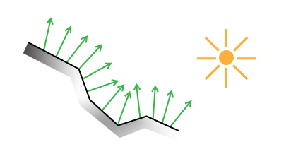
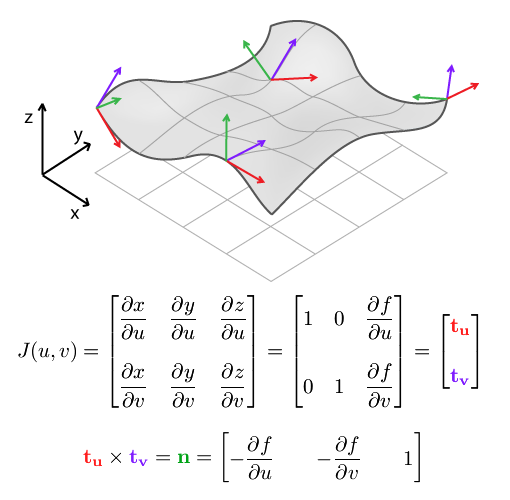
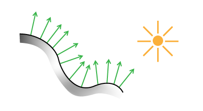
Lighting a surface using its normals.
</p>

<p>
To use normals for lighting, I have two options. The first is to do this on a geometry basis, assigning a normal to every triangle in the planet mesh. This is straightforward, but ties the quality of the shading to the level of detail in the geometry. A second, better way is to use a normal map. You stretch an image over the surface, as you would for applying textures, but instead of color, each pixel in the image represents a normal vector in 3D. Each pixel's channels (red, green, blue) are used to describe the vector's X, Y and Z values. When lighting the surface, the normal for a particular point is found by looking it up in the normal map.
</p>

<p>
The benefit of this approach is that you can stretch a high resolution normal map over low resolution geometry, often with almost no visual difference.
</p>

<p class="tc">
<img class="natural" src="/files/making-worlds/planet-3-normal-lighting-simple.png" alt="Schematic representation of surface shading with normals" />
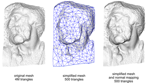
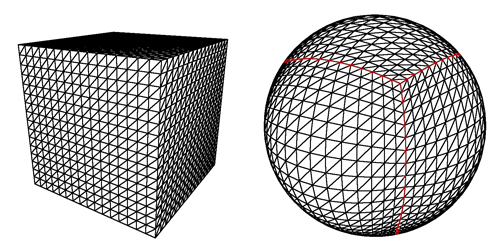
Lighting a low-resolution surface using high-resolution normals.
</p>

<p>
Here's the technique applied to a real model:
</p>

<p class="tc">
<img class="natural" src="/files/making-worlds/planet-3-normal-mapping-3d.png" alt="Normal mapping in practice" />
(<a href="http://en.wikipedia.org/wiki/File:Normal_map_example.png">Source</a> - Creative Commons Share-alike Attribution)
</p>

<p>
Normal mapping helps keep performance up and memory usage down.
</p>

<h3>Finding Normals</h3>

<p>
So how do you generate such a normal map, or even a single normal at a single point? There are many ways, but the basic principle is usually the same. First you calculate two different vectors which are tangent to the surface at the point in question. Then you use the <a href="http://en.wikipedia.org/wiki/Cross_product">cross product</a> to find a vector perpendicular to the two. This third vector is unique and will be the surface normal.
</p>

<p>
For triangles, you can pick any two triangle edges as vectors. In my case, the surface is described by a heightmap on a sphere, which makes things a bit trickier and requires some math.
</p>

<p>
I asked my friend <a href="http://twitter.com/mathseeker">Djun Kim</a>, Ph.D. and teacher of mathematics at UBC for help and he recommended <a href="http://en.wikipedia.org/wiki/Calculus_on_Manifolds_(book)">Calculus on Manifolds</a> by Michael Spivak. This deceptively small and thin book covers all the basics of calculus in a dense and compact way, and quickly became my new favorite reading material.
</p>

<h2>Differential Geometry</h2>

<p>
In this section, I'll describe the formulas needed to calculate the normals of a spherical heightmap. Unlike what I've written before, this will dive shamelessly into specifics and not eschew math. The reason I'm writing it down is because I couldn't find a complete reference online. If math scares you, this section might not be for you. Scroll down until you reach the crater, or take a detour by reading <a href="http://www.maa.org/devlin/LockhartsLament.pdf">A Mathematician's Lament</a> by Paul Lockhart, which will enlighten you.
</p>

<p>
First, we're going to derive normals for a regular flat terrain heightmap. To start, we need to define the terrain surface. Starting with a 2D heightmap, i.e. a function <em>f(u,v)</em> of two coordinates that returns a height value, we can create a 3 dimensional surface <em>g</em>:
</p>

<p>
<img class="natural" src="/files/making-worlds/planet-3-terrain-mapping.png" alt="Mathematical formulation of heightmapping" />
</p>

<p>
We can use this formal description to find tangent and normal vectors. A vector is tangent when its direction matches the slope of the surface in a particular direction. Differential math tells us that slope is found by taking the derivative. For our function of 2 variables, that means we can find tangent vectors along curves of constant <em>v</em> or constant <em>u</em>. These curves are the thin grid lines in the diagram. Actually, we can find tangents along any line, in any direction. But along <em>u</em> and <em>v</em> lines, the other variable acts like a constant, which simplifies things.
</p>

<p>
To do this, we take partial derivatives with respect to <em>u</em> (with <em>v</em> constant) and with respect to <em>v</em> (with <em>u</em> constant). The set of all partial derivatives is called the Jacobian matrix J, whose rows form the tangent vectors <b>t<sub>u</sub></b> and <b>t<sub>v</sub></b>, indicated in red and purple:
</p>

<p>
<img class="natural" src="/files/making-worlds/planet-3-terrain-mapping-jacobian.png" alt="Heightmapping, jacobian, finding normals" />
</p>

<p>
The cross product of <b>t<sub>u</sub></b> and <b>t<sub>v</sub></b> gives us <b>n</b>, the surface normal.
</p>

<p>
When applied to a discrete heightmap, the function <em>f(u,v)</em> is a 2D array <em>map[u][v]</em>, and the partial derivatives at the end have to be replaced with something else. We can use <a href="http://en.wikipedia.org/wiki/Finite_difference">finite differences</a> to approximate the slope of the surface by differencing neighbouring samples:
</p>

<p>
  <img class="natural" src="/files/making-worlds/finite-diff.png" alt="Finite differences" /><br />
<img class="natural" src="/files/making-worlds/planet-3-terrain-mapping-finite-diff.png" alt="Heightmapping, finite differences" />
</p>

<p>
This result and the formula for <b>n</b> are usually provided as-is in terrain mapping guides, without going through the full process of finding tangents first. However, it's important to use the Jacobian matrix formulation once you switch to spherical terrain.
</p>

<p>
<img class="natural" src="/files/making-worlds/planets-1-cubemap.png" alt="Mapping a cube to a sphere" />
</p>

<p>
To make a sphere, we add an additional function <em>k</em> which warps the flat terrain into a spherical shell. Each shell is the result of warping a single face of the cubemap and covers exactly 1/6th of the sphere. In what follows, We'll only consider a single face and its shell.
</p>

<p>
We designate the intermediate pre-warp coordinates <em>(s,t,h)</em>, and the final post-warp coordinates as <em>(x,y,z)</em>:
</p>

<p>
<img class="natural" src="/files/making-worlds/planet-3-sphere-mapping.png" alt="Mathematical formulation of spherical heightmapping" />
</p>

<p>
The principle behind the spherical mapping is this: first we take the vector <em>(s, t, 1)</em>, which lies in the base plane of the flat terrain. We normalize this vector by dividing it by its length <em>w</em>, which has the effect of projecting it onto the sphere: <em>(s/w, t/w, 1/w)</em> will be at unit distance from <em>(0, 0, 0)</em>. Then we multiply the resulting vector by the terrain height <em>h</em> to create the terrain on the sphere's surface, relative to its center: <em>(h&middot;s/w, h&middot;t/w, h/w)</em>
</p>

<p>
Just like with the function <em>g(u,v)</em> and <em>J(u,v)</em>, we can find the Jacobian matrix <em>J(s,t,h)</em> of <em>k(s,t,h)</em>. Because there are 3 input values for the function <em>k</em>, there are 3 tangents, along curves of varying <em>s</em> (with constant <em>t and h</em>), varying <em>t</em> (constant <em>s and h</em>) and varying <em>h</em> (constant <em>s and t</em>). The three tangents are named <b>t<sub>s</sub></b>, <b>t<sub>t</sub></b>, <b>t<sub>h</sub></b>.
</p>

<p class="tc">
<img class="natural" src="/files/making-worlds/planet-3-sphere-mapping-jacobian.png" alt="Spherical heightmapping, jacobian." />
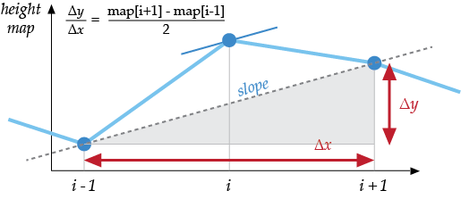
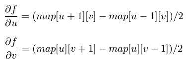
PS: If your skills at derivation are a bit rusty, remember that <a href="http://www.wolframalpha.com/input/?i=d%2Fdx+h%2Fsqrt%28x%5E2%2By%5E2%2B1%29">Wolfram Alpha can do it for you</a>.
</p>

<p>
How does this help? The three vectors describe a local frame of reference at each point in space. Near the edges of the grid, they get more skewed and angular. We use these vectors to transform the flat frame of reference into the right shape, so we can construct a new 90 degree angle here.
</p>

<p>
In mathematical terms, we multiply the 'flat' partial derivatives by the Jacobian matrix. This is similar to the chain rule for regular derivatives, only for multiple variables.
</p>

<p>
That is, to find the partial derivatives (i.e. tangent vectors) of the final spherical terrain with respect to the original terrain coordinates <em>u</em> and <em>v</em>, we can take the flat terrain's tangents <b>t<sub>u</sub></b> and <b>t<sub>v</sub></b> and multiply them by <em>J(s,t,h)</em>. Once we have the two post-warp tangents, we take their cross product, and find the normal of the spherical terrain:
</p>

<p>
<img class="natural" src="/files/making-worlds/planet-3-sphere-mapping-normal.png" alt="Spherical heightmapping, jacobian." />
</p>

<p>
It's imporant to note that this is not the same as simply multiplying the flat terrain normal with <em>J(s,t,h)</em>. <em>J(s,t,h)</em>'s rows do not form a set of perpendicular vectors (it is not an orthogonal matrix), which means it does not preserve angles between vectors when you multiply by it. In other words, <em>J(s,t,h) * n</em>, with n the flat terrain normal, would not be perpendicular to the spherical terrain. This is why it's important to return to the basic calculus underneath, so we can get the correct, complete formula.
</p>

<p>
Thus ends the magical math adventure. If you read it all the way through, cheers!
</p>

<h2>No Wait, It is a Moon.</h2>

<p>
With the normal map in place, I can now render the planet's surface and get a realistic idea of what it looks like. To show this off, I tweaked the brush system a bit: instead of using the literal brush image (e.g. a smooth, round crater), the brush is distorted with fractal noise. It makes every application of the brush subtly different from the next, and saves me from manually drawing e.g. a hundred different craters.
</p>

<p class="tc">
<img class="natural" src="/files/making-worlds/planet-3-brush-distortion.png" alt="Brush distortion." /><br />
Here's a side by side comparison of the original brush and a distorted version.
</p>

<p>
Currently I've only implemented one type of distortion, which lends a rocky appearance to the surface. With that in place, my engine can now generate somewhat realistic looking moon surfaces. Here's the demo:
</p>

<p>
  <iframe style="margin: 0 auto;" width="560" height="380" src="https://www.youtube.com/embed/pHjyMs8tm4E" frameborder="0" allowfullscreen="allowfullscreen"></iframe>
</p>

<h3>References</h3>

<p>
The techniques I used were pioneered by people smarter and older than me, I'm just building my own little digital machine with them.
</p>

<ul>
<li><a href="http://www.cs.cmu.edu/~ajw/s2007/0251-SphericalWorlds.pdf">Creating Spherical Worlds</a>, Maxis/Electronic Arts. (<a href="http://www.andrewwillmott.com/s2007">source</a>).</li>
<li><a href="http://en.wikipedia.org/wiki/Calculus_on_Manifolds_(book)">Calculus on Manifolds</a>, Michael Spivak.</li>
</ul>

</div></div>
]]></content>
  </entry>
  
</feed>
