<cartesian>
  …
  <interval expression="..." />
  <line />
</cartesian>

expression: function (x, i, emit) {
  y = Math.sin(x + time) + … ;
  emit(x, y);   
},
// typedArray[p++] = x;
// typedArray[p++] = y;

<spherical>
  <area items="2" expression="..." />
  <lerp items="32" />
  <vector />
</spherical>

  expression: function (x, y, i, j, emit) {
    ...
    emit(x, y, z);
    emit(x + a * r, y + b * r, z + c * r);
  },
  

<cartesian>
  <interval history="96" id="woosh" expression="..." />
  <transpose order="xwzy" />
  <vector />

  <transpose order="ywzx" source="#woosh" />
  <vector />
</cartesian>

<cartesian> <grid /> </cartesian>

<rtt>
  <cartesian> <grid /> </cartesian>
</rtt>
<compose />

<area expression="..." />
<compose />

<rtt>
  <compose color="#fcfbfa" />
  <cartesian> <grid /> </cartesian>
</rtt>
<compose />

<rtt history="2">
  <remap shader="..." />
  <compose />
  <cartesian> <grid /> </cartesian>
</rtt>
<compose />

vec4 getSample(vec3 xyz);
vec4 getFramesSample(vec3 xyz) {
  vec4 c = getSample(xyz + vec3( 0.0, 0.0, 1.0));
  vec3 t = getSample(xyz + vec3( 0.0, 1.0, 0.0)).xyz;
  vec3 b = getSample(xyz + vec3( 0.0,-1.0, 0.0)).xyz;
  vec3 l = getSample(xyz + vec3(-1.0, 0.0, 0.0)).xyz;
  vec3 r = getSample(xyz + vec3( 1.0, 0.0, 0.0)).xyz;
  return vec4((t + b + l + r) / 2.0 - c.xyz, c.w);
}

<rtt>
  …
</rtt>
<lerp />
<remap shader="..." />
<vector />

…
vec3 _sn_1_truncateVec(vec4 v) { return v.xyz; }
vec4 _sn_6_getFramesSample(vec3 xyz) {
  vec4 c = _sn_6_getSample(xyz + vec3( 0.0, 0.0, 1.0));
  vec3 t = _sn_6_getSample(xyz + vec3( 0.0, 1.0, 0.0)).xyz;
  vec3 b = _sn_6_getSample(xyz + vec3( 0.0,-1.0, 0.0)).xyz;
  vec3 l = _sn_6_getSample(xyz + vec3(-1.0, 0.0, 0.0)).xyz;
  vec3 r = _sn_6_getSample(xyz + vec3( 1.0, 0.0, 0.0)).xyz;
  return vec4((t + b + l + r) / 2.0 - c.xyz, c.w);
}
vec4 _pg_2_(vec4 _io_1_v) {
  vec3 _io_2_return;
  vec4 _io_15_return;

  _io_2_return = _sn_1_truncateVec(_io_1_v);
  _io_15_return = _sn_6_getFramesSample(_io_2_return);
  return _io_15_return;
}

Notes will appear here.
Please view in Chrome or Firefox. Chrome is glitchy, Firefox is stuttery. Work in progress. :/

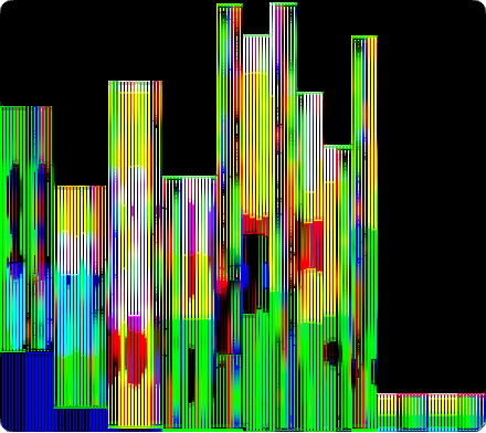
This is my website, Acko.net. Which you may know as that site with that header, made with WebGL, using Three.js.

The entire effect is based on Vertex Displacement, applied on the GPU.
If I disable the part of the vertex shader that fetches the position, only a static mesh is left.

It's more accurate to call it Vertex Replacement. The actual positions, normals and occlusion are read from a texture, indexed by the mesh. The texture can be updated independently of the underlying draw call. This nicely separates the how from the what.

It's an indirection with an associated cost, but you gain something very valuable: random access to all your geometry data.

Specifically, it enables you to emulate Geometry Shaders on WebGL 1, a feature we won't get until WebGL 3. Also transform feedback. Today, in a browser, on a phone.

For the past year, I've been exploring how to apply this principle in general and at scale. The result is MathBox 2. Still incomplete, but already showing some very neat behavior.

Education is the art of conveying a sense of truth by telling a series of decreasing lies. In order to explain MathBox 2, I'm going to use some creative license.

MathBox 2 enables Data Driven Geometry. When I say it's "somewhat like D3 but for WebGL", that's a good introduction, but not very accurate.

MathBox is like a better SVG. It aims to be a better fit for data visualization.

See, if you want to render this simple graph with SVG, you need 1 path but 32 circles.

Which means you need a completely different tree structure depending on the choice of representation (line or points).
Libraries like D3 contain helpers to make this easier, but it's still a very leaky abstraction.

In MathBox, I separate the data from the representation. Here I use an interval along which I sample an expression 32 times. An interval is just a fancy array with sampling behavior. It's rendered as lines and points, but there's only one line node and one point node.
Nodes combine like lego to form visible objects.

Note the XML is just a helpful notation, MathBox is not XML based, but it does have a DOM just like XML / HTML.

The goal of MathBox is to be O(1) Box. It shouldn't matter how many of something you draw. 1 is as simple as 100. Or 100 × 100. Or 100 × 100 × 100.
Insert giant asterisk here.

It supports offloading complicated computations to the GPU. Like projecting native 4D points to 3D, tesselating them into lines and surfaces, and differentiating them on the fly. Here I'm drawing distorted toruses using the Hopf Fibration of the 3-Sphere. Trust me, this is good math porn.

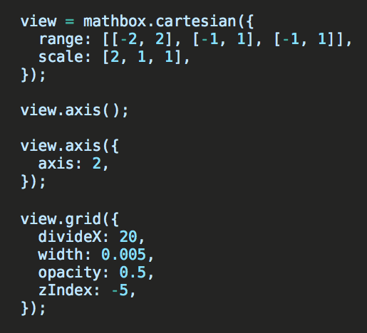
So what does the code actually look like? Take this simple graph: a rectangular or cartesian grid, with axes, and a moving curve on top.

It's created just using some JavaScript, passing in a set of properties for each node. It's generous in what it accepts (e.g. CSS colors), but strict in what it stores: each property has a type and canonical representation. The properties are still somewhat in flux, so don't stare yourself blind.

I'm going to pretend it is XML and only highlight the relevant properties. It's easier because it's familiar.
You can see how the MathBox DOM is a tree, but with composition between siblings, not just parents and children.

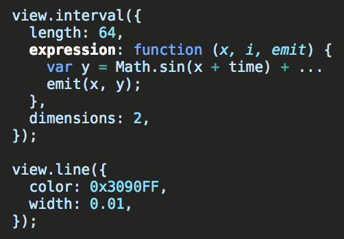
The curve renders live data, provided by a JS expression. It's a function of one variable x (and the array index i). But rather than returning values, you emit them. This emit() call streams the arguments into a typed array of floats. It's very optimizable, and profiling shows it's not that far from native floating point performance. This is the only real O(n) JS code in the entire visualization, everything else is O(1).

Once filled, the array is uploaded to GPU memory. The new data is automatically used to produce the next frame. The best two-way data binding is just two pointers to the same piece of memory.

Changing a property on a node (like a color) works similarly. Three.js manages shader uniforms using {value: x} objects. These can be shared by reference like registers, bound directly to specific DOM node attributes. Change a node, and all its Three.js materials update instantly. No cascade required.

Here's a more interesting example: two spherical clouds of vectors. Note the vectors are curved, not straight. Scroll to zoom.

For each cloud, I sample a 2D area with an expression. Each iteration produces two items: the start and end point of each vector. Hence this is really a 2+1D array: N × N × 2. The array is linearly interpolated (lerp) to N × N × 32, then rendered as polyline vectors in spherical coordinates.

The expression is now a function of x and y (indices i and j), and it emits two points per call.

But each point is itself a 3D vector. So it's really an N × N × 32 × 3 array. Remember what I said about lies.

Again, it's all done on the GPU: tessellating points into lines into triangle strips, placing and orienting the cones, cutting off the (curved) polyline where the arrow begins, etc. In fact, the lines are sized in a hybrid 2.5D fashion to enhance the line-art quality. It's more sophisticated than it might seem.

These arrays can do more tricks, for example they support history. Here I'm filling a 2D array of points, one row at a time. This is really just a cyclic buffer. The data sampling shader scrolls through the data virtually, without being aware of it.

History is simple, just set history: N. Each array is secretly always 4D (or 5D if you're picky), opening up its extra dimensions as needed. 4 is the max today, for technical reasons.

Here I'm actually drawing two renderables from a single data source, transposed differently in each case. I use a CSS selector #woosh to link to the source the 2nd time, similar to anchor tags.

The <vector> doesn't care what it's rendering from. It just samples an abstract data source at certain coordinates. The sophisticated polyline arrow behavior still works.

What you're really doing is building shaders and draw calls automatically. Which operate on giant arrays that may only exist as transient values deep inside a GPU core. Memory bandwidth is the biggest bottleneck there, so this is usually a net win, despite the 'wasteful' repeated computation.

There's still a static geometry template of course, created once on init per renderable, but it doesn't change, just like Acko.net's header.

It goes beyond just math diagrams though. Here I'm rendering two scenes on top of each other, with a gradient blended on top.

This is done using the render-to-texture operator, <rtt>. It renders whatever's inside to a texture. The RTT acts as just another data source, which can be piped into a <compose>. This is a full screen drawing pass. Document order is drawing order.

You can also pipe a regular array into <compose>, that's how the gradient works.

This is where this model really starts to show some surprising expressivity. All drawables support blend modes, so this is already ridiculously close to a generic effects composer.

For example, nothing needs to be added to support framebuffer feedback.

This is because the auto-linking behavior extends to parents too. If you place a naked compose directly inside an RTT, it links up with its parent, rendering the output back as input the next frame. Here I'm applying a fade out by setting the inner compose's color to slightly less than white.

It just works because the RTT is automatically double buffered, creating a read and write target, doing the swapping for you.

In fact, I only needed to add a single operator to do this classic demoscene water effect. This is a discrete approximation of the Navier-Stokes equation, for shallow surface waves.

It uses the remap operator. It applies a sampling kernel, supplied as a GLSL shader. RTT also supports history, so when you set history: 2, you get a triple buffered render target: two read buffers, and one write buffer.

The shader is vanilla GLSL, but with one twist: it declares and uses a function getSample without a body. This callback is linked in for you, allowing you to sample anything without having to care how. The render target is exposed as a single N x N x 2 volume texture, despite the constant buffer swapping.

By adding only three operators: RTT, compose and remap, MathBox has suddenly turned into Winamp AVS or Milkdrop.

You could do all of this by hand of course, this is old school GPGPU... But all the tedious set up and state management has been abstracted for you.

For example, this is something I threw together in 15 minutes. It uses the same simple fluid solver, but creates resonant waves with an additional rotozoomer movement, finishing off with a color map. This is 3 remaps and 3 RTTs, set up as a directed cyclic graph.

What I've shown you is pretty much all the major pieces I have today. It's definitely incomplete, and significant parts around it are missing (e.g. tracked animations, camera nodes, html/text overlays, slides director, etc). So you'll have to use your imagination to see where this can really go.

In this example, I'm rendering to a texture just like before, but I'm not composing it into the scene. Instead I'm rendering the texture as a grid of 3D vectors.

It works, because RTT is just a data source.

Now imagine what happens when you add audio input... or audio output. Or maybe physics, so you can do force-directed layout on the GPU.

The secret sauce behind all of this is ShaderGraph 2. It's a functional GLSL linker/recompiler. It's a total rewrite of ShaderGraph 1, powering MathBox 1.

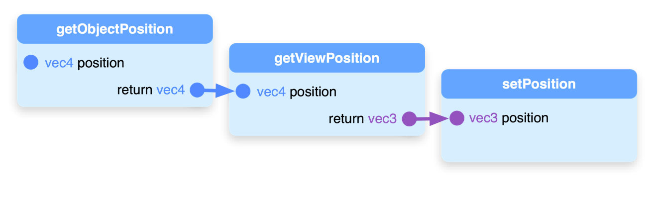
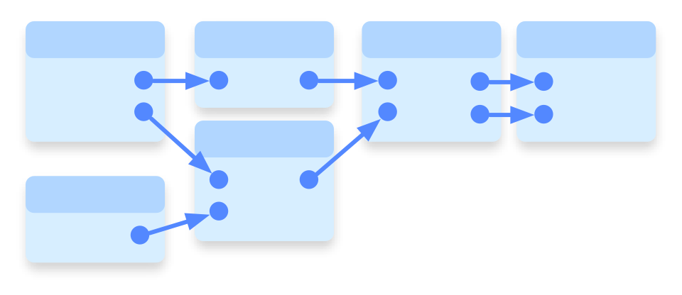
ShaderGraph 1 could link up snippets of GLSL into pipelines, by matching type signatures. This is just a simple one-input one-output scenario.

You could construct arbitrary directed acyclic graphs out of snippets, which got compiled into a single vertex and fragment shader. It's driven by code though, it's not a graphical UI.

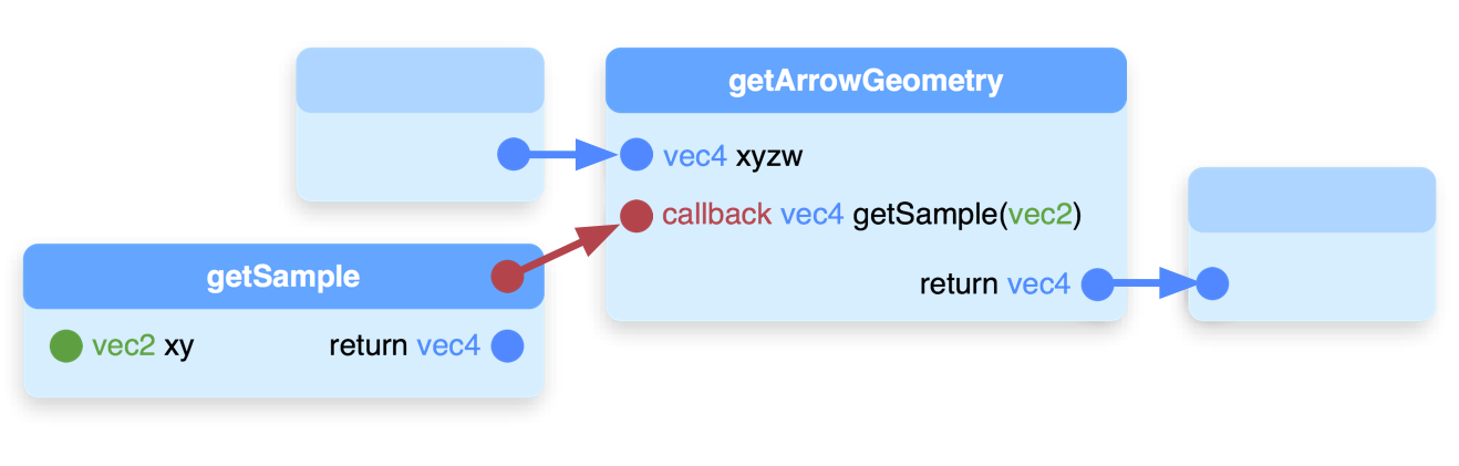
ShaderGraph 2 fixes some bad design decisions, and adds one major change: callbacks. It turns the traditional data flow into something functional, allowing e.g. the getArrowGeometry shader to call getSample as much as it wants. The data flow is essentially redirected to a completely different part of the graph.

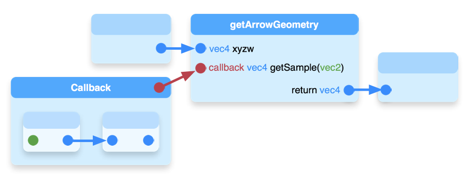
But callbacks can be graphs themselves. Any open inputs or outputs are bundled up into its type signature. This is what allows complicated behavior to be wrapped up and re-used in a completely modular fashion.

The output looks like this, though this is only part of a (fragment) shader. You can recognize the sampling kernel from earlier, whose global symbols have been namespaced to avoid collisions. You can also see _pg_2_, a generated program that calls two functions in order and returns the result.

Using ShaderGraph 2's chainable factory API, partially built shaders can be passed around and extended in a completely agnostic fashion. Shader uniforms can be instanced too, binding unique parameters to each instance. You only need to agree on a type signature between partners. It's fast too, compiling a shader in a few milliseconds if the cache is warm, or a few tens of ms when cold.

In summary: MathBox 2 is a reactive DOM for data visualization. It lets you stream data into virtual geometry shaders and more, offloading various computations to the GPU. It's built as an extensible, multi-layered architecture on top of Three.js which I won't go into yet, but suffice it to say, it is not as opaque as presented here. I hope to release MathBox 2 before the end of the year, and ShaderGraph 2 sooner. MathBox 2 is out!

Diagrams powered by MathBox 2 alpha.

Use Ctrl/Cmd + or Ctrl/Cmd - to size to fit.

‹ ›